Unique values for an array of n rows and m columns

XcelLearner

Board Regular
Joined
Feb 6, 2016
Messages
52
Office Version
  1. 365
  2. 2016
Platform
  1. Windows
Hi,

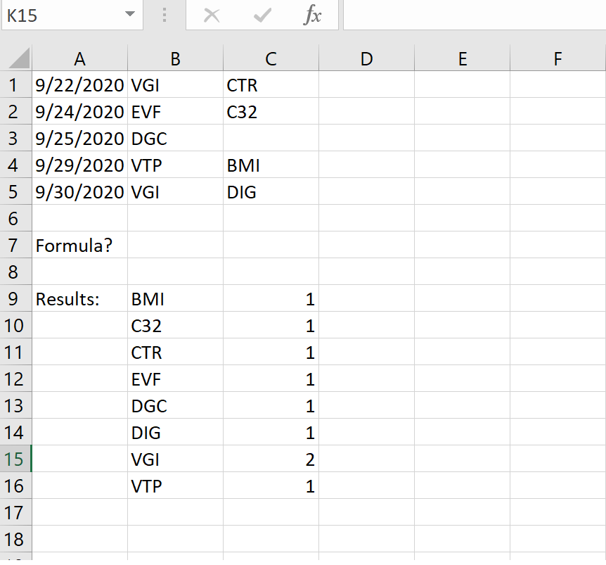
I have a table of n rows and m columns. For simplicity, I use a table of 5 rows and 2 columns from B1:C5. I try to find unique values, filtering for blank value (as in C3). I look for a formula that extracts values from both columns and rows - I googled for the usage of UNIQUE function but it seems that solutions are based on either rows or columns, not both. I would also like to count the times of appearance for each unique value.

The expected results would be in B9:B16 for unique values, and C9:C16 for counts.
cKXVUTm.png


Can anyone please help with the formula? I am using Office 365. Thanks a lot.
 

Excel Facts

Can Excel fill bagel flavors?
You can teach Excel a new custom list. Type the list in cells, File, Options, Advanced, Edit Custom Lists, Import, OK
Function UNIQUE won't work for a block of values, just a row or a column. The solution is to stack all the column sections into one column and then use UNIQUE. One way is complex formulas. The best way to do it is PowerQuery.

Watch this ExcelIsFun video and see if it helps.
 
Upvote 0
I have Excel 365, but my company has been agonizingly slow in getting it updated to include the new dynamic array functions. So I wrote some UDFs to emulate the functionality. They are of course not exact, so whatever I try may not work on the actual functions. But given that try these 2 formulas:

B9:
Excel Formula:
=SORT(UNIQUE(INDEX(B1:C5,MOD(SEQUENCE(10,,0),5)+1,INT(SEQUENCE(10,,0)/5)+1)))
C9:
Excel Formula:
=COUNTIF(B1:C5,B9#)
 
Upvote 0
Good show, Eric! I tinkered with the spilling formulas and came up with this. The blanks are irritating, but I kept experimenting and just used FILTER to rid the array of them. These columns and rows have to be contiguous for this type of approach to work.

MrExcel posts18.xlsx
BC
2itemAitemB
3ae
4bf
5cf
6dg
7h
8e
9ai
10
11
12unique list, sortedcount of items
13a2
14b1
15c1
16d1
17e2
18f2
19g1
20h1
21i1
22
Sheet52
Cell Formulas
RangeFormula
B13:B21B13=FILTER(SORT(UNIQUE(INDEX(B3:C9,MOD(SEQUENCE(ROWS(B3:C9)*COLUMNS(B3:C9),,0),ROWS(B3:C9))+1,INT(SEQUENCE(ROWS(B3:C9)*COLUMNS(B3:C9),,0)/ROWS(B3:C9))+1))),SORT(UNIQUE(INDEX(B3:C9,MOD(SEQUENCE(ROWS(B3:C9)*COLUMNS(B3:C9),,0),ROWS(B3:C9))+1,INT(SEQUENCE(ROWS(B3:C9)*COLUMNS(B3:C9),,0)/ROWS(B3:C9))+1)))<>0)
C13:C21C13=COUNTIF($B$3:$C$9,B13#)
Dynamic array formulas.
 
Last edited:
Upvote 0
A few other 'spill' options ..
- G2 if the range is not too big. The issue with the size of the range is that the REPT(" ",100) may have to be increased and in any case if the range is fairly larger the character limit for TEXTJOIN (32,767) may get exceeded & the formula will fail
- For larger ranges, or in any case, if you also have the new LET function try the I2 formula. This could still exceed the TEXTJOIN limit but should handle a much larger range before failing.
- If you do not have the LET function, J2 contains the same formula but without the shortenings enabled by LET

In all cases the spilling COUNTIF formula already suggested is still applicable.

I note also that the OP's results are sorted but there was no mention of that requirement so I have not sorted. Any of my formulas could be wrapped in a SORT function if required though.

20 10 29.xlsm
BCDEFGHIJ
1ListCountListList
2PlumPlum2PlumPlum
3PlumWatermelonAppleMelonWatermelon1WatermelonWatermelon
4MelonKiwifruitBlackberryApple2AppleApple
5RaspberryMelonAppleMelonMelon4MelonMelon
6Kiwifruit1KiwifruitKiwifruit
7Blackberry1BlackberryBlackberry
8Raspberry1RaspberryRaspberry
9
Unique Count 1
Cell Formulas
RangeFormula
G2:G8G2=UNIQUE(TRIM(MID(TEXTJOIN(REPT(" ",100),1,IF(B2:E5="","",B2:E5)),SEQUENCE(COUNTA(B2:E5),,1,100),100)))
H2:H8H2=COUNTIF(B2:E5,G2#)
I2:I8I2=LET(Cnt,COUNTA(B2:E5),TxtJ,"|"&TEXTJOIN("|",1,IF(B2:E5="","",B2:E5))&"|",Seq,SEQUENCE(Cnt),Subs,SUBSTITUTE(SUBSTITUTE(TxtJ,"|","#",Seq),"|","%",Seq),UNIQUE(REPLACE(LEFT(TxtJ,FIND("%",Subs)-1),1,FIND("#",Subs),"")))
J2:J8J2=UNIQUE(REPLACE(LEFT("|"&TEXTJOIN("|",1,IF(B2:E5="","",B2:E5))&"|",FIND("%",SUBSTITUTE(SUBSTITUTE("|"&TEXTJOIN("|",1,IF(B2:E5="","",B2:E5))&"|","|","#",SEQUENCE(COUNTA(B2:E5))),"|","%",SEQUENCE(COUNTA(B2:E5))))-1),1,FIND("#",SUBSTITUTE(SUBSTITUTE("|"&TEXTJOIN("|",1,IF(B2:E5="","",B2:E5))&"|","|","#",SEQUENCE(COUNTA(B2:E5))),"|","%",SEQUENCE(COUNTA(B2:E5)))),""))
Dynamic array formulas.
 
Last edited:
Upvote 0
Don, thanks for working out the details! I'd hoped that SORT might sort the empty cells to the end, but I guess not. The FILTER works, although it essentially doubles the size of the formula. Maybe using LET could help. I think this could work on some non-contiguous ranges. For example, if the columns are A1:A5 C1:C5, and E1:E5, you'd give INDEX the range A1:E5, and multiply the results of the INT portion by 2 (more or less). Still awkward, and there still would be limitations, but possible.

Peter, clever use of TEXTJOIN! A neat way to compress a 2-d text array to 1-d. The OP's original list is not quite sorted (EVF is out of place), but I think that was the intent.
 
Upvote 0
I have Excel 365, but my company has been agonizingly slow in getting it updated to include the new dynamic array functions. So I wrote some UDFs to emulate the functionality. They are of course not exact, so whatever I try may not work on the actual functions. But given that try these 2 formulas:

B9:
Excel Formula:
=SORT(UNIQUE(INDEX(B1:C5,MOD(SEQUENCE(10,,0),5)+1,INT(SEQUENCE(10,,0)/5)+1)))
C9:
Excel Formula:
=COUNTIF(B1:C5,B9#)
Thanks a lot, Eric. Your formulas work, except that they don't filter the blank cells. Appreciate.
By the way, I am testing your formulas, and see that the first formula works with small range. As I have a larger data set, I revise the "10" to "1000" and it seems to work well.
 
Upvote 0
Thanks a lot, Eric. Your formulas work, except that they don't filter the blank cells. Appreciate.
By the way, I am testing your formulas, and see that the first formula works with small range. As I have a larger data set, I revise the "10" to "1000" and it seems to work well.
The 10 represents 2 columns times 5 rows = 10. The 5 in the formula is the number of rows. So adjust it to your range accordingly. If you look at DRSteele's post (#4), he adjusted my original formula to figure out the number of rows and columns based on the range you use. So you don't need to figure out the row/column values, just put the range in all 14 places in the formula. He also added the FILTER function to remove blank cells.

Glad we could help!
 
Upvote 0
Thank you very much for your helps, Eric, Don, and Peter.

I tested three formulas (actually four, as Peter generously offered several options), and I've found that all approaches give consistent results. (Must be so, but it is still amazing for me, haha.) While Eric's and Don's solutions are a bit comprehensible for me, Peter's are things that I've seen first time. I like Peter's, because they look shorter (especially the I2 formula), though I don't understand how they work.
Thanks a lot for your time. Have a great day.

I might tweak the problem a bit, just for curiosity, but I need to work on those given formulas first.
 
Upvote 0
You're welcome. You ended up with quite a lot of choice.
So just to confuse you some more, here is yet another one that is a bit shorter again (provide you have LET) and does not have the potential problem with TEXTJOIN that my other formulas had. :)

20 10 29.xlsm
BCDEFG
1List
2PlumPlum
3PlumWatermelonAppleMelonWatermelon
4MelonKiwifruitBlackberryApple
5RaspberryMelonAppleMelonMelon
6Kiwifruit
7Blackberry
8Raspberry
9
Unique Count 1
Cell Formulas
RangeFormula
G2:G8G2=LET(Agg,AGGREGATE(15,6,((ROW(B2:E5)-ROW(B2)+1)*10^6+COLUMN(B2:E5)-COLUMN(B2)+1)/(B2:E5<>""),SEQUENCE(COUNTA(B2:E5))),UNIQUE(INDEX(B2:E5,Agg/10^6,RIGHT(Agg,6))))
Dynamic array formulas.
 
Upvote 0

Forum statistics

Threads
1,214,585
Messages
6,120,399
Members
448,958
Latest member
Hat4Life

We've detected that you are using an adblocker.

We have a great community of people providing Excel help here, but the hosting costs are enormous. You can help keep this site running by allowing ads on MrExcel.com.
Allow Ads at MrExcel

Which adblocker are you using?

Disable AdBlock

Follow these easy steps to disable AdBlock

1)Click on the icon in the browser’s toolbar.
2)Click on the icon in the browser’s toolbar.
2)Click on the "Pause on this site" option.
Go back

Disable AdBlock Plus

Follow these easy steps to disable AdBlock Plus

1)Click on the icon in the browser’s toolbar.
2)Click on the toggle to disable it for "mrexcel.com".
Go back

Disable uBlock Origin

Follow these easy steps to disable uBlock Origin

1)Click on the icon in the browser’s toolbar.
2)Click on the "Power" button.
3)Click on the "Refresh" button.
Go back

Disable uBlock

Follow these easy steps to disable uBlock

1)Click on the icon in the browser’s toolbar.
2)Click on the "Power" button.
3)Click on the "Refresh" button.
Go back
Back
Top