Unique values for an array of n rows and m columns

XcelLearner

Board Regular
Joined
Feb 6, 2016
Messages
52
Office Version
  1. 365
  2. 2016
Platform
  1. Windows
Hi,

I have a table of n rows and m columns. For simplicity, I use a table of 5 rows and 2 columns from B1:C5. I try to find unique values, filtering for blank value (as in C3). I look for a formula that extracts values from both columns and rows - I googled for the usage of UNIQUE function but it seems that solutions are based on either rows or columns, not both. I would also like to count the times of appearance for each unique value.

The expected results would be in B9:B16 for unique values, and C9:C16 for counts.

cKXVUTm.png


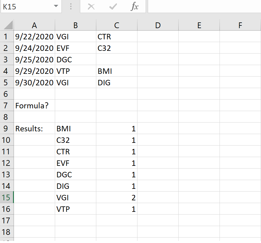
Can anyone please help with the formula? I am using Office 365. Thanks a lot.
 
So just to confuse you some more, here is yet another one that is a bit shorter again (provide you have LET) and does not have the potential problem with TEXTJOIN that my other formulas had.
Best version yet! I especially like how you can use AGGREGATE to add additional conditions to exclude values if desired.

Here's another shorter version using LET:

Excel Formula:
=LET(r,ROWS(B2:E5),seq,SEQUENCE(r*COLUMNS(B2:E5),,0),arr,INDEX(B2:E5,MOD(seq,r)+1,seq/r+1),UNIQUE(FILTER(arr,arr<>0)))

Regrettably, I still don't have the ability to test it.
 
Upvote 0

Excel Facts

Excel Wisdom
Using a mouse in Excel is the work equivalent of wearing a lanyard when you first get to college
That works for me
+Fluff v2.xlsm
ABCDEFGH
1PeterEric
2PlumPlumPlum
3PlumWatermelonAppleMelonWatermelonMelon
4MelonKiwifruitBlackberryAppleRaspberry
5RaspberryMelonAppleMelonMelonWatermelon
6KiwifruitKiwifruit
7BlackberryApple
8RaspberryBlackberry
9
Sheet2
Cell Formulas
RangeFormula
G2:G8G2=LET(Agg,AGGREGATE(15,6,((ROW(B2:E5)-ROW(B2)+1)*10^6+COLUMN(B2:E5)-COLUMN(B2)+1)/(B2:E5<>""),SEQUENCE(COUNTA(B2:E5))),UNIQUE(INDEX(B2:E5,Agg/10^6,RIGHT(Agg,6))))
H2:H8H2=LET(r,ROWS(B2:E5),seq,SEQUENCE(r*COLUMNS(B2:E5),,0),arr,INDEX(B2:E5,MOD(seq,r)+1,seq/r+1),UNIQUE(FILTER(arr,arr<>0)))
Dynamic array formulas.
 
Upvote 0
Hi

Also a solution if you can't (won't) use the new functions.
I used Peter's layout and values. With F1 empty or with a value not in the target range, in F2:

Excel Formula:
=IFERROR(INDIRECT(TEXT(MIN(IF($A$2:$D$5<>"",IF(ISERROR(MATCH($A$2:$D$5,$F$1:F1,0)),100000*ROW($A$2:$D$5)+COLUMN($A$2:$D$5)))),"\R0\C00000"),FALSE),"")

This is an array formula, you have to confirm it with CTRL-SHIFT-ENTER
Copy down
 
Last edited:
Upvote 0
This is an array formula, you have to confirm it with CTRL-SHIFT-ENTER
To clarify, in the case of the OP, who apparently has the new array functions, C+S+E confirmation is not required
Great idea for the problem though!

I also like Eric's latest 'LET' formula. (y)

But since we have been continually shortening the formulas, all the previous LET formulas can be shortened a tiny bit further with one more assignment pair. Here is Eric's with that addition
Excel Formula:
=LET(a,B2:E5,r,ROWS(a),seq,SEQUENCE(r*COLUMNS(a),,0),arr,INDEX(a,MOD(seq,r)+1,seq/r+1),UNIQUE(FILTER(arr,arr<>0)))

? .. and if we wanted to be pedantic, not including reducing all the variable names to single characters, one more character could be saved by changing the value of seq from
SEQUENCE(r*COLUMNS(a),,0)
to
SEQUENCE(r*COLUMNS(a))-1
.. though I believe that does make the calculation a little less efficient so not worth it anyway. :(
 
Upvote 0
Solution
I like Peter's addition, not just for the shortness, but because it is easier to maintain. In this version, the range only has to be entered 1 time instead of 3. Less chance for someone to miss one.

I thought of a way to shorten it by 2 characters (without changing variable names):

Excel Formula:
=LET(a,B2:E5,r,ROWS(a),seq,SEQUENCE(r*COLUMNS(a),,r),arr,INDEX(a,MOD(seq,r)+1,seq/r),UNIQUE(FILTER(arr,arr<>0)))

and this actually might make it a tad more efficient, but I still prefer the previous version. I like the symmetry of the +1, +1 and I think it makes the formula easier to understand. Which raises another point. This is a fairly complicated formula, but with proper use of LET, I think it's pretty easy to see what it's doing. I think that's really more valuable than the reduction in size.
 
Upvote 0
Greetings
this works for Office 2019
What about this, Feedback Please
I have this unique but sorted from Lowest to highest
Press CTRL+SHIFT+ENTER to enter array formulas.

MREXCEL.xlsx
ABC
1DATEITEMS
29/22/2020VGICTR
39/24/2020EVFC32
49/25/2020DGC
59/29/2020VTPBMI
69/30/2020VGIDIG
7
8
9
10ITEMSQnt
11BMI1
12C321
13CTR1
14**DGC1
15DIG1
16**EVF1
17VGI2
18VTP1
19  
Unique values for an array of n
Cell Formulas
RangeFormula
B11:B19B11=IFERROR(INDEX($B$2:$C$6,MOD(MATCH(1,(FILTERXML("<t><s>"&SUBSTITUTE(TEXTJOIN("/",FALSE,SUBSTITUTE(COUNTIF($B$2:$C$6,"<"&TRANSPOSE($B$2:$C$6)),";",",")),"/","</s><s>")&"</s></t>","//s[count(node())>0]")+(--FILTERXML("<t><s>"&SUBSTITUTE(TEXTJOIN("/",FALSE,SUBSTITUTE(TRANSPOSE($B$2:$C$6<>""),";",",")),"/","</s><s>")&"</s></t>","//s[count(node())>0]")))-SUM(COUNTIF($B$2:$C$6,B$10:B10)),0)-1,ROWS($B$2:$C$6))+1,CEILING(MATCH(1,(FILTERXML("<t><s>"&SUBSTITUTE(TEXTJOIN("/",FALSE,SUBSTITUTE(COUNTIF($B$2:$C$6,"<"&TRANSPOSE($B$2:$C$6)),";",",")),"/","</s><s>")&"</s></t>","//s[count(node())>0]")+(--FILTERXML("<t><s>"&SUBSTITUTE(TEXTJOIN("/",FALSE,SUBSTITUTE(TRANSPOSE($B$2:$C$6<>""),";",",")),"/","</s><s>")&"</s></t>","//s[count(node())>0]")))-SUM(COUNTIF($B$2:$C$6,B$10:B10)),0),ROWS($B$2:$C$6))/ROWS($B$2:$C$6)),"")
C11:C19C11=IF(B11<>"",COUNTIF($B$2:$C$6,B11),"")
Press CTRL+SHIFT+ENTER to enter array formulas.
 
Upvote 0
... with proper use of LET, I think it's pretty easy to see what it's doing. I think that's really more valuable than the reduction in size.
I agree with both points. :biggrin:
 
Upvote 0
Thank you very much to all of you for a very lively discussion. I benefit a lot, though I don't understand much of the formulae. For me, many formulae are ones I first saw, and I've tried all of them.
For Dossfm0q's solution, I couldn't make it to work, even when I was mindful for a CSE. I CSE'ed and dragged down but it didn't come out with with same output with other formulae.

To clarify, in the case of the OP, who apparently has the new array functions, C+S+E confirmation is not required
Great idea for the problem though!

I also like Eric's latest 'LET' formula. (y)

But since we have been continually shortening the formulas, all the previous LET formulas can be shortened a tiny bit further with one more assignment pair. Here is Eric's with that addition
Excel Formula:
=LET(a,B2:E5,r,ROWS(a),seq,SEQUENCE(r*COLUMNS(a),,0),arr,INDEX(a,MOD(seq,r)+1,seq/r+1),UNIQUE(FILTER(arr,arr<>0)))

? .. and if we wanted to be pedantic, not including reducing all the variable names to single characters, one more character could be saved by changing the value of seq from
SEQUENCE(r*COLUMNS(a),,0)
to
SEQUENCE(r*COLUMNS(a))-1
.. though I believe that does make the calculation a little less efficient so not worth it anyway. :(
If we all agree, I will choose the solution submitted by Peter, revised from Eric's as the best solution. It is like a team work.
 
Upvote 0
another approach
DateValue1Value2ValueCount
9/22/2020VGICTRBMI1
9/24/2020EVFC32C321
9/25/2020DGCCTR1
9/29/2020VTPBMIDGC1
9/30/2020VGIDIGDIG1
EVF1
VGI2
VTP1

Power Query:
let
    Source = Excel.CurrentWorkbook(){[Name="Table4"]}[Content],
    RC = Table.RemoveColumns(Source,{"Date"}),
    Unpivot = Table.UnpivotOtherColumns(RC, {}, "Attribute", "Value"),
    TSC = Table.SelectColumns(Unpivot,{"Value"}),
    Group = Table.Group(TSC, {"Value"}, {{"Count", each Table.RowCount(_), type number}}),
    Sort = Table.Sort(Group,{{"Value", Order.Ascending}})
in
    Sort
 
Upvote 0

Forum statistics

Threads
1,214,542
Messages
6,120,116
Members
448,945
Latest member
Vmanchoppy

We've detected that you are using an adblocker.

We have a great community of people providing Excel help here, but the hosting costs are enormous. You can help keep this site running by allowing ads on MrExcel.com.
Allow Ads at MrExcel

Which adblocker are you using?

Disable AdBlock

Follow these easy steps to disable AdBlock

1)Click on the icon in the browser’s toolbar.
2)Click on the icon in the browser’s toolbar.
2)Click on the "Pause on this site" option.
Go back

Disable AdBlock Plus

Follow these easy steps to disable AdBlock Plus

1)Click on the icon in the browser’s toolbar.
2)Click on the toggle to disable it for "mrexcel.com".
Go back

Disable uBlock Origin

Follow these easy steps to disable uBlock Origin

1)Click on the icon in the browser’s toolbar.
2)Click on the "Power" button.
3)Click on the "Refresh" button.
Go back

Disable uBlock

Follow these easy steps to disable uBlock

1)Click on the icon in the browser’s toolbar.
2)Click on the "Power" button.
3)Click on the "Refresh" button.
Go back
Back
Top