Use a formula to populate names based on text in cells

[Gummyworms1234]

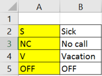
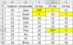
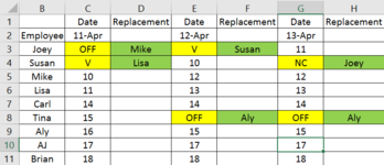
I am working on our employee schedules for next week and I have an issue. I want to make names appear under the replacement column automatically without having to type it in or write it in each time an employee won’t be working. I made an example of what I am looking for and highlighted the specific cells I am looking at. On the sheet1 picture, I’ve highlighted a few possible messages that I can use when an employee isn’t working. On the sheet2 picture, I’ve shown on April 11th Joey has an off day and Susan is on vacation. Mike and Lisa told me they can cover for them. I want to make Mike and Lisa’s names appear on our sign in sheet since I have OFF and V on April 11th. I’d like Mike and Lisa’s name to appear under the replacement column like I’ve shown on the sheet3 picture. If someone can help me with this issue I have, I’d appreciate it!

 

[hajiali]

do you have a sheet/place on any sheet that Identifies Mike and Lisa will be the replacements? or do you have any notation any where were they replace them?

 

[Gummyworms1234]

do you have a sheet/place on any sheet that Identifies Mike and Lisa will be the replacements? or do you have any notation any where were they replace them?

I’m somewhat confused by what you’re trying to ask. On sheet2 of my spreadsheet, I identify that Mike and Lisa will be the replacement because they have the location number associated with Joey and Susan. Hopefully that answers you question. From what I’ve read online, I think an index formula or vlookup formula would be what I need.

 

[hajiali]

Ok I think this is what you want assuming that in sheet 3 Column A you have the location number as well. If so try this in Cell D3 and drag the formula down

Cell D3=IFERROR(IF(NOT(ISNUMBER(C3)),INDEX(Sheet2!$B$2:$B$21,MATCH(A3,Sheet2!$C$2:$C$21,0)),""),"")

 

[Gummyworms1234]

Ok I think this is what you want assuming that in sheet 3 Column A you have the location number as well. If so try this in Cell D3 and drag the formula down

Cell D3=IFERROR(IF(NOT(ISNUMBER(C3)),INDEX(Sheet2!$B$2:$B$21,MATCH(A3,Sheet2!$C$2:$C$21,0)),""),"")

This formula worked for columb D on sheet 3. So if I want to

Ok I think this is what you want assuming that in sheet 3 Column A you have the location number as well. If so try this in Cell D3 and drag the formula down

Cell D3=IFERROR(IF(NOT(ISNUMBER(C3)),INDEX(Sheet2!$B$2:$B$21,MATCH(A3,Sheet2!$C$2:$C$21,0)),""),"")

This formula was what I needed for the example spreadsheet and it works on my main spreadsheet I'm using for my schedules! Thanks for the help!!

 

[hajiali]

Glad I could help.