I was able to get an interesting workaround for icon sets with three icons, having to do with both number and conditional formatting.
First, set the number format for positive, negative, and zero values as follows:
- Under Format Cells, under the Number tab, select Custom.
- Type the text values you want to use in the Type box in this order: "highest";"lowest";"middle". These correspond to formatting for positive, negative and zero values, respectively.
- Press OK.
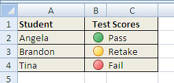
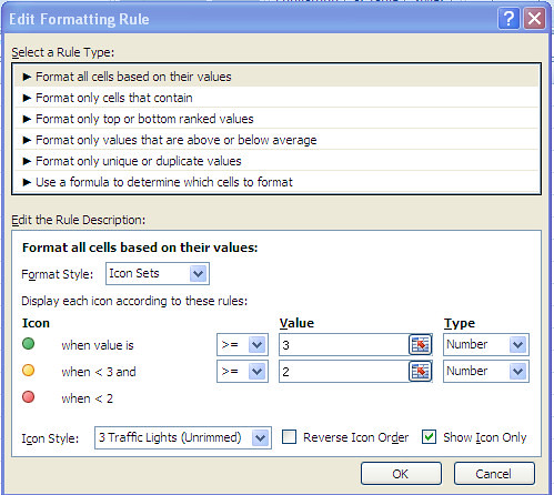
You can then fill the original text values with positive, negative and zero values as required by your spreadsheet. Then, apply your conditional formatting with the icon sets, using the Formula option to set the first icon for positive values, the second for zero values and the third for negative values. Your icons and text should show up in a single cell.