Using INDEX and MATCH that reference multiple drop-down lists

[Legacy 479016]

I have drafted a monthly report which has a main dashboard sheet, along with monthly report sheet (the plan is to add additional sheets as the months progress).


Within the dashboard sheet I have a summary, so every time I select a name from a drop-down it displays key data pulled from the monthly sheet. The function to achieve this looks like this:

=INDEX(April21!E$2:E$36,MATCH(F3,April21!A$2:A$36,0))

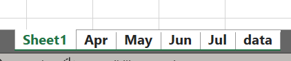
So F3 is the drop-down list in my dashboard sheet, and it is pulling data from the April21 sheet.


My question is this: Can I reference multiple drop-down lists within this function? If I select a name from the first drop-down list, then the month from a second drop-down list, it will show the data for that name from that month.


Any assistance would be most appreciated.

 

[AhoyNC]

With Excel 365 you could use the FILTER function.
In the example below F2 and G2 would be your drop down lists.

Book1
	A	B	C	D	E	F	G
1	Name	Month	Amount			From Drop	Down
2	Name11	April	100			Name11	May
3	Name12	April	101			103
4	Name12	May	102
5	Name11	May	103
6	Name15	May	104
7	Name11	June	105
8	Name11	July	106
Sheet1

Cell Formulas
Range	Formula
F3	F3	=FILTER(C2:C8,($A$2:$A$8=$F$2)*($B$2:$B$8=$G$2),"No Data")

 

[Legacy 479016]

With Excel 365 you could use the FILTER function.
In the example below F2 and G2 would be your drop down lists.

Book1
	A	B	C	D	E	F	G
1	Name	Month	Amount			From Drop	Down
2	Name11	April	100			Name11	May
3	Name12	April	101			103
4	Name12	May	102
5	Name11	May	103
6	Name15	May	104
7	Name11	June	105
8	Name11	July	106
Sheet1

Cell Formulas
Range	Formula
F3	F3	=FILTER(C2:C8,($A$2:$A$8=$F$2)*($B$2:$B$8=$G$2),"No Data")

Many thanks for assistance. I have managed to get the first half working, however the second part is a challenge. Let me explain...

So for the first part:

=FILTER(April21!$E$2:$E$36,(April21!$A$2:$A$36=$F$3)

This works. However the second part (which references the second drop-down list) doesnt work:

=FILTER(April21!E$2:E$36,(April21!$A$2:$A$36=$F$3)*(May21!E$2:E$36,(May21!$A$2:$A$36=$W$3)))

Any thoughts please?

 

[AhoyNC]

The syntax in the last part of your formula (in red below) is wrong
FILTER(April21!E$2:E$36,(April21!$A$2:$A$36=$F$3)*(May21!E$2:E$36,(May21!$A$2:$A$36=$W$3)))
What is this part of the formula trying to do?
(May21!E$2:E$36,(May21!$A$2:$A$36=$W$3))
Are you trying to get two different sets of data from sheets April21 and May21? If so, what do you want to do with this data when it is retrieved?
Can you post a small sample of your data and the expected results?

 

[Legacy 479016]

The syntax in the last part of your formula (in red below) is wrong
FILTER(April21!E$2:E$36,(April21!$A$2:$A$36=$F$3)*(May21!E$2:E$36,(May21!$A$2:$A$36=$W$3)))
What is this part of the formula trying to do?
(May21!E$2:E$36,(May21!$A$2:$A$36=$W$3))
Are you trying to get two different sets of data from sheets April21 and May21? If so, what do you want to do with this data when it is retrieved?
Can you post a small sample of your data and the expected results?

As per the mini-sheet below, I have sheet 1 with 2 drop-down lists (cells B1 and B2). When I select a name, columns 1-4 below are populated by the data in the Apr sheet (see attached screenshot for workbook structure).

What I want to do is: When I select a name AND a month from the 2 drop-down lists, the data for the selected name is displayed from the corresponding months worksheet.

FYI - all tables listed in the 'month' worksheets have the same structure and position.

I hope this makes more sense.

Book1.xlsx
	A	B	C	D
1	Name	name4
2	Date
3
4
5
6	Col1	Col2	Col3	Col4
7	55	7	8	9
8
Sheet1

Cell Formulas
Range	Formula
A7:D7	A7	=FILTER(Apr!B$2:B$5,(Apr!$A$2:$A$5=$B$1))

Cells with Data Validation
Cell	Allow	Criteria
B1	List	=data!$A$1:$A$4
B2	List	=data!$C$1:$C$4

 

[AhoyNC]

See if this works for you.
Enter the formula in A7 and the answers should spill into the other columns.
The INDIRECT function should find the right sheet for each month.
Change cell references to match your data.

Book3
	A	B	C	D
1	Name	name4
2	Date	Apr21
3
4
5
6	Col1	Col2	Col3	Col4
7	55	7	8	9
Sheet1

Cell Formulas
Range	Formula
A7:D7	A7	=FILTER(INDIRECT($B$2&"!$B$2:$E$5"),INDIRECT($B$2&"!$A$2:$A$5")=$B$1)
Dynamic array formulas.

Apr21 sheet

Book3
	A	B	C	D	E
1	Name
2	Name1	50	32	34	18
3	Name2	25	21	49	34
4	Name3	36	18	18	29
5	Name4	55	7	8	9
Apr21