Hi guys,
I have a very complicated question that I need help with.
Basically, I am trying to work out the potential customers for suburbs based on their distance to other suburbs and the rules that apply. So in short:
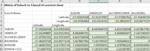
1. Need to work out a suburbs distance from one to another (e.g. Annerley to Bardon) that is located on another sheet (all distances have already been calculated between suburbs).
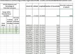
2. Then use that to apply the rules which is (if a suburb is within 2km of one another then it is 5% of potential customers)
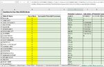
3. The potential customers for each suburb are also on another sheet.
So for example:
Albion to Annerley is 4km, which means Albion is only entitled to receive 5% of the potential customers from Annerley (where Annerley has 4579 customers. So it would be 5% of that figure. I have something that is close but is not returning a true value (e.g. if suburbs are over 5km away, they receive 0%, so answer should be 0) but mine is not returning that.
This is what I have:
=IFERROR(VLOOKUP(INDEX('Matrix of Suburb Distances'!$A$3:$AM$43,MATCH($A4,'Matrix of Suburb Distances'!$A$3:$A$43,0),MATCH(E$3,'Matrix of Suburb Distances'!$A$3:$AM$3,0)),Constant!$AD$6:$AE$9,2,TRUE),Constant!$AE$6)*VLOOKUP($A4,Constant!$AG:$AK,COLUMNS(Constant!$AG$3:$AK$3),0)
Any help would be appreciated
I have a very complicated question that I need help with.
Basically, I am trying to work out the potential customers for suburbs based on their distance to other suburbs and the rules that apply. So in short:
1. Need to work out a suburbs distance from one to another (e.g. Annerley to Bardon) that is located on another sheet (all distances have already been calculated between suburbs).
2. Then use that to apply the rules which is (if a suburb is within 2km of one another then it is 5% of potential customers)
3. The potential customers for each suburb are also on another sheet.
So for example:
Albion to Annerley is 4km, which means Albion is only entitled to receive 5% of the potential customers from Annerley (where Annerley has 4579 customers. So it would be 5% of that figure. I have something that is close but is not returning a true value (e.g. if suburbs are over 5km away, they receive 0%, so answer should be 0) but mine is not returning that.
This is what I have:
=IFERROR(VLOOKUP(INDEX('Matrix of Suburb Distances'!$A$3:$AM$43,MATCH($A4,'Matrix of Suburb Distances'!$A$3:$A$43,0),MATCH(E$3,'Matrix of Suburb Distances'!$A$3:$AM$3,0)),Constant!$AD$6:$AE$9,2,TRUE),Constant!$AE$6)*VLOOKUP($A4,Constant!$AG:$AK,COLUMNS(Constant!$AG$3:$AK$3),0)
Any help would be appreciated