using SEQUENCE to spill the content of a single cell over a range

Youngling

New Member
Joined
Mar 11, 2021
Messages
7
Office Version
  1. 365
Platform
  1. MacOS
Setting
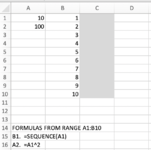
Suppose I want to have the numbers from 1 to 10 generated in the range B1:B10. I can store N in A1 and type =SEQUENCE(A1) in B1. A dynamic array is generated that gets the job done.

My problem
I have an arbitrary computation in A2 that I want to copy 10 times in the range C1:C10. I want to be able to use dynamic arrays somehow, in such a way that: (a) I type some formula in C1, (b) this formula reads the "10" in A1, and the content of A2 is automatically copied in the range C1:C10. I want the solution to be so that, if I change A1 to, say, 20, the range where A2 is 'spilled' into is automatically adjusted to be C1:C20.

I do not want to use VBA to solve the problem.

I'm using Microsoft 365 (Excel 16.46.21021202) on a MacBook Pro (2019) running Catalina (10.15.7).

Any help would be greatly appreciated.
 

Attachments

  • Screen Shot 2021-03-11 at 9.01.02 AM.png
    Screen Shot 2021-03-11 at 9.01.02 AM.png
    160.9 KB · Views: 21

Excel Facts

Lock one reference in a formula
Need 1 part of a formula to always point to the same range? use $ signs: $V$2:$Z$99 will always point to V2:Z99, even after copying
Is this what you mean?

Book1 (version 1).xlsb
ABC
120100
2100101
3102
4103
5104
6105
7106
8107
9108
10109
11110
12111
13112
14113
15114
16115
17116
18117
19118
20119
Sheet3
Cell Formulas
RangeFormula
C1:C20C1=SEQUENCE(A1,1,A2)
Dynamic array formulas.
 
Upvote 0
Solution
Hi & welcome to MrExcel.
Maybe one of these
+Fluff 1.xlsm
ABCD
11011100
210024100
339100
4416100
5525100
6636100
7749100
8864100
9981100
1010100100
11
Stock
Cell Formulas
RangeFormula
B1:B10B1=SEQUENCE(A1)
C1:C10C1=B1#^2
D1:D10D1=IF(B1#,A2)
A2A2=A1^2
Dynamic array formulas.
 
Upvote 0
No, but your answer gave me the idea to get what I first wanted: =SEQUENCE(A1,,A2,0). Very grateful, thank you.

Which brings me to my next question: suppose that A2 contains the formula = A1 * RAND(). Then using my solution above =SEQUENCE(A1,,A2,0) yields a dynamic array of constant numbers. If I hit 'recalculate' the numbers are updated but they're all the same. My hope was that every time the number got 'copied' down, that the machine would recalculate, so that I would end up getting . This is, for example, what would happen if I used the DATA TABLE array formula {=TABLE(,A3)} in C2:C10. In a sense, I am hoping to replace that DATA TABLE command with something that was dynamic.
 
Upvote 0
I've never used Data tables so have no idea what you are trying to do, but the reason all your values are the same is that you have used a step of 0 in the formula.
 
Upvote 0
The following mini may clarify matters further. I want 10 'copies' of what is in B6. If I use =SEQUENCE(B2,,B6,0) in cell D2 I get my ten copies (in range D2 to D11). But they are 'the same.' If I refer to B6 in E2 and then use {=TABLE(,C1)} in cells E3:E11 I get my ten 'independent and identically distributed' copies, using the data table array formula, which is what I want, but then if I change the number of copies to, say, 20, in B2, i'd have to reprogram the data table. I'm trying to accomplish what the data table does in this example with dynamic arrays so that the size of the array is dynamic.

Book4
ABCDE
1X + YX + Y
2Trials10-0.3473319-0.3473319
3Variable X-0.571409186-0.3473319-0.1615321
4Variable Y0.224077303-0.3473319-1.2400353
5-0.3473319-1.3728739
6X + Y-0.347331883-0.3473319-0.1272208
7-0.34733193.44566243
8-0.3473319-3.473457
9-0.34733190.23469291
10-0.34733190.60382376
11-0.3473319-2.8717248
Sheet2
Cell Formulas
RangeFormula
D2:D11D2=SEQUENCE(B2,,B6,0)
B3B3=NORM.S.INV(RAND())
B4B4=T.INV(RAND(),2)
B6B6=SUM(B3:B4)
E2E2=B3+B4
E3:E11E3=TABLE(,C1)
Press CTRL+SHIFT+ENTER to enter array formulas.
Dynamic array formulas.
 
Upvote 0
Have you looked at the RANDARRAY function?

Yes, I have looked at RANDARRAY. Thank you. It does what I need if I can 'bake' all my computations in cell D2 (in my example above I would type =NORM.S.INV(RANDARRAY(B2))+T.INV(RANDARRAY(B2),2) in cell D2), but sometimes that is unwieldy, in such a way that I want to be able to simply refer to cells that then get recalculated, as in my data table example.
 
Upvote 0
Since my original questions was answered I will close this thread and ask my updated question in a new post. Thank you everybody!!
 
Upvote 0

Forum statistics

Threads
1,214,591
Messages
6,120,432
Members
448,961
Latest member
nzskater

We've detected that you are using an adblocker.

We have a great community of people providing Excel help here, but the hosting costs are enormous. You can help keep this site running by allowing ads on MrExcel.com.
Allow Ads at MrExcel

Which adblocker are you using?

Disable AdBlock

Follow these easy steps to disable AdBlock

1)Click on the icon in the browser’s toolbar.
2)Click on the icon in the browser’s toolbar.
2)Click on the "Pause on this site" option.
Go back

Disable AdBlock Plus

Follow these easy steps to disable AdBlock Plus

1)Click on the icon in the browser’s toolbar.
2)Click on the toggle to disable it for "mrexcel.com".
Go back

Disable uBlock Origin

Follow these easy steps to disable uBlock Origin

1)Click on the icon in the browser’s toolbar.
2)Click on the "Power" button.
3)Click on the "Refresh" button.
Go back

Disable uBlock

Follow these easy steps to disable uBlock

1)Click on the icon in the browser’s toolbar.
2)Click on the "Power" button.
3)Click on the "Refresh" button.
Go back
Back
Top