Using SumIFS with Index and Match

[Peter Davison]

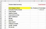
I have an "output" file where I want to sum sales based on a cell criteria. My sum values are in the Performance Sheet C2:C200000. My criteria could be 1 of many which is in cell B4 selected from a lookup list. The data is in another file in the Product Sheet in a range of Cells C1:Z500 (Headings that relate to cell B4 are in Row1 but could be in any column). I have a list of attributes associated with B4 in cells B5 to B15. My formula is in C5 to start with and will then be copied down to the other cells C6 to C15.
The formula below is returning "VALUE" I think I have something wrong in the last part of the formula C1:Z500, but I'm not sure what it needs to be?

I would appreciate any help you can give me please.

=SUMIFS(INDEX('[Breakfast Foods Combined Raw Data.xlsx]Performance Data'!$C$2:$C$200000,,MATCH($B$4,'[Breakfast Foods Combined Raw Data.xlsx]Product Data'!$C$1:$Z$1,0)),'[Breakfast Foods Combined Raw Data.xlsx]Product Data'!$C$1:$Z$500,"="&$B5)

 

[Anthony47]

If the interval to be summed is on rows $2:$200000 then the criteria interval should similarly be 199999 lines long (ie cannot be $C$1:$Z$500)
Also, INDEX needs as first parametre an array (multi column) whereas you use a single column list ( $C$2:$C$200000)

Bye

 

[Peter Davison]

Thank you for your help.
It has been really very helpful.

I do have another query that I sent in the other day that no one has replied, I wondered if you would be able to help. (See below)


I'm trying to set a dynamic range in a chart
My header is in cell E16 and my data can be in cells E17 to E517 or more
For this example my data is only 200 cells created from formulas in the cells so I have 300 blank cells with formulas in.
I don't know how to make the dynamic range ignore the formula blank cells?
Any help would be appreciated.
Thanks

=OFFSET('Start Data1'!$E$16,0,0,COUNTA('Start Data1'!$E$17:$E$517)-1,1)

 

[Anthony47]

You refer to Using Offset and CountA to create a dynamic range in a chart

I posted a suggestion in that discussion

Bye