Using SUMPRODUCT and ISNUMBER to find if an array of number has a number included with special conditions

[Lekazard]

I'm banging my head with this issue and help would be highly appreciated.
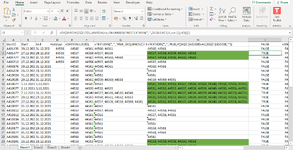
I have some data gathered monthly and to sum it up I need to discover if midweek holidays are included within a range of dates. For simplicity the relevant data on the sheet is structured like this:

D: Dates I'm comparing	H: Date range	I: Expected output values
44536	44531; 44532; 44533; 44537; 44538; 44539; 44540	FALSE
44556	44531; 44532; 44533; 44537; 44538; 44539; 44540; 44550; 44551; 44552; 44553	FALSE
44559	44531; 44532; 44533; 44537; 44538; 44539; 44540; 44550; 44551; 44552; 44553; 44557; 44558; 44559; 44560; 44561	TRUE

What I want to know is does the the array listed in column H have any of the numbers listed in column D with the special rule there must be one consecutive datevalue before and 2 after (to simplify, if the number we are comparing is 2, then an array of 1, 2, 3, 4 would give TRUE).
The two formulas I've tried to use in column I are:
=IF(AND(ISNUMBER(MATCH(D2-1; $H$2:$H$1000; 0)); OR(ISNUMBER(MATCH(D2+2; $H$2:$H$1000; 0)); ISNUMBER(MATCH(D2+3; $H$2:$H$1000; 0)))); TRUE; FALSE)
and
=IF(SUMPRODUCT(--(ISNUMBER(MATCH(D2:D1000-1; $H$2:$H$1000; 0))); --(ISNUMBER(MATCH(D2:D1000+2; $H$2:$H$1000; 0))); --(ISNUMBER(MATCH(D2:D1000+3; $H$2:$H$1000; 0)))) > 0; TRUE; FALSE)
but both give FAIL for every row meaning, that they are not compiled right. Because of localization I use semicolon as the separator inside formulas. Could anyone help me out with this one because my head is really starting to hurt.

 

[Fluff]

Ok what does this return

=SUM(--(CODE(MID(H4,SEQUENCE(LEN(H4)),1))>59))

Change the H4 to a cell that should return true.

 

[Lekazard]

Ok what does this return

=SUM(--(CODE(MID(H4,SEQUENCE(LEN(H4)),1))>59))

Change the H4 to a cell that should return true.

I pasted it into I4 and then used the Fill Handle for every row. For every row it returns 0

 

[Fluff]

In that case I'm not sure why it's not working for you, I though you might have some non-breakin spaces, but obviously not.
As can be seen in both posts#3 & 4 those suggestions work for us.
Can you copy the data we posted into a blank sheet, change the commas to semi-colons & see if that works.
To copy the data use the copy icon

 

[Peter_SSs]

I'm guessing that if the previous suggestions have not worked for you then this probably won't either, but this is how I would attempt it.

Lekazard.xlsm
	D				H	I
1
2	44536				44531; 44532; 44533; 44537; 44538; 44539; 44540	FALSE
3	44556				44531; 44532; 44533; 44537; 44538; 44539; 44540; 44550; 44551; 44552; 44553	FALSE
4	44559				44531; 44532; 44533; 44537; 44538; 44539; 44540; 44550; 44551; 44552; 44553; 44557; 44558; 44559; 44560; 44561	TRUE
Sheet1

Cell Formulas
Range	Formula
I2:I4	I2	=ISNUMBER(FIND(TEXTJOIN("; ",,SEQUENCE(4,,D2-1)),H2))

 

[kvsrinivasamurthy]

Is it possible to upload sample file in some website and give link here.

 

[Lekazard]

Is it possible to upload sample file in some website and give link here.

WPS 365

eu.docworkspace.com

Here's the data and some of the formulas I've been trying. The layout of the sheets is pretty awful but hopefully it's readable. Also last thing I tried was VBA, but couldn't get the out come with that method either.

Sub CheckConsecutiveAndSecondPosition()
    Dim arr() As String
    Dim rngD As Range
    Dim cellD As Range
    Dim i As Long
    Dim matchCount As Integer
    
    ' Get the values in column D
    Set rngD = Range("D2:D" & Cells(Rows.Count, "D").End(xlUp).Row)
    
    ' Clean and split the array in cell H14 by semicolon
    arr = Split(Replace(Trim(Range("H14").Value), ";", " "), " ")
    
    ' Initialize match count
    matchCount = 0
    
    ' Check if any number in column D matches the conditions
    For Each cellD In rngD
        If IsNumeric(cellD.Value) Then
            For i = 0 To UBound(arr) - 3
                If CLng(Val(arr(i))) = cellD.Value And _
                    IsNumeric(arr(i + 1)) And CLng(Val(arr(i + 1))) = cellD.Value - 1 And _
                    IsNumeric(arr(i + 2)) And CLng(Val(arr(i + 2))) = cellD.Value + 1 And _
                    IsNumeric(arr(i + 3)) And CLng(Val(arr(i + 3))) = cellD.Value + 2 Then
                    matchCount = matchCount + 1
                    Exit For
                End If
            Next i
        End If
    Next cellD
    
    ' Set the boolean output based on the match count
    Range("I14").Value = (matchCount > 0)
End Sub

 

[Peter_SSs]

I didn't understand the requirement before. I think that I do now. How is this?

23 06 03.xlsm
	D				H	I
1	Holidays				44560; 44561	FALSE
2	44558				44560; 44561	FALSE
3	44536				44557; 44558; 44559; 44560; 44561	TRUE
4	44556				44557; 44558; 44559; 44560; 44561	TRUE
5	44559				44557; 44558	FALSE
6					44560; 44561	FALSE
7					44553	FALSE
8					44561	FALSE
9					44559; 44560; 44561	FALSE
10					44531; 44532; 44533; 44537; 44538; 44539; 44540; 44550; 44551; 44552; 44553; 44557; 44558; 44559; 44560; 44561	TRUE
Check sequence

Cell Formulas
Range	Formula
I1:I10	I1	=OR(BYROW(D$2:D$5,LAMBDA(rw,ISNUMBER(FIND(TEXTJOIN("; ",,SEQUENCE(4,,rw-1)),H1)))))

 

[Lekazard]

I didn't understand the requirement before. I think that I do now. How is this?

23 06 03.xlsm
	D				H	I
1	Holidays				44560; 44561	FALSE
2	44558				44560; 44561	FALSE
3	44536				44557; 44558; 44559; 44560; 44561	TRUE
4	44556				44557; 44558; 44559; 44560; 44561	TRUE
5	44559				44557; 44558	FALSE
6					44560; 44561	FALSE
7					44553	FALSE
8					44561	FALSE
9					44559; 44560; 44561	FALSE
10					44531; 44532; 44533; 44537; 44538; 44539; 44540; 44550; 44551; 44552; 44553; 44557; 44558; 44559; 44560; 44561	TRUE
Check sequence

Cell Formulas
Range	Formula
I1:I10	I1	=OR(BYROW(D$2:D$5,LAMBDA(rw,ISNUMBER(FIND(TEXTJOIN("; ",,SEQUENCE(4,,rw-1)),H1)))))

I copy-pasted this formula into my sheet, and this is the first formula which gave me the expected output! It works! Still gotta do some testing on Monday and I have couple of more conditions I need to apply and take under consideration, but this was by far the hardest part of this task and now after being stuck for over a week I can now proceed further.

Big thanks for everyone giving a helping hand, can't state how much I appreciate this!

 

[Peter_SSs]

You're welcome. Glad we could help. Thanks for the follow-up.