Values-specific coloured cells to retain its colour

Joined
May 20, 2021
Messages
26
Office Version
  1. 2016
Platform
  1. Windows
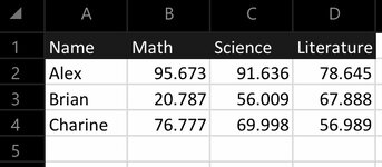
Sheet 1: Has values like 33.878 in Yellow, 17.873 in Red and 96.666 in Green.

Is there a way to ensure that these coloured cells are carried over to sheet 2? (Sheet 2 has a macro that sorts out the scores according to percentile and other considerations so I can’t just copy&paste/use simple filtering or sorting and was wondering if there is a code to bring the colours-specific to its value over instead of manually colouring them)
 

Excel Facts

Ambidextrous Undo
Undo last command with Ctrl+Z or Alt+Backspace. If you use the Undo icon in the QAT, open the drop-down arrow to undo up to 100 steps.
"33.878 in Yellow" to me means in yellow font. Later you say "coloured cells" which to me means cells filled with a color.
Which of the two is it?
You could try
Code:
If c.Value = 33.878 Then c.Font.Color = ??????   "<------ whatever colour
ElseIf c.Value = 17.873 Then c.Font.Color = ??????   "<------ whatever colour
ElseIf c.Value = 96.666 Then c.Font.Color = ??????   "<------Whatever colour
End If
 
Upvote 0
"33.878 in Yellow" to me means in yellow font. Later you say "coloured cells" which to me means cells filled with a color.
Which of the two is it?
You could try
Code:
If c.Value = 33.878 Then c.Font.Color = ??????   "<------ whatever colour
ElseIf c.Value = 17.873 Then c.Font.Color = ??????   "<------ whatever colour
ElseIf c.Value = 96.666 Then c.Font.Color = ??????   "<------Whatever colour
End If
My apologies, I meant coloured cells.

Sheet 1 has hundreds of unique numbers with their own cell colour, is there a way to just tag the value to its cell colour so that it reflects on sheet 2 even if the numbers are rearranged?
 
Upvote 0
"even if the numbers are rearranged" in Sheet1 or Sheet2?

Don't quote if not absolutely required. Just a bunch of extra clutter
 
Upvote 0
Sorry, new to this, thanks for the advice.

So in Sheet 1, it is just a chunk of unsorted data detailing the scores of each student like in the image attached. I did not colour the cells in the image but the values all have their own cell colours. (Green, Orange, Yellow, Red) I do not know how they categorise the colours, it is not based on percentile.

In Sheet 2, after a bunch of macros that I am unable to access (confidentiality so even I am left out of it), they are all sorted out according to which students are in the A band, B band and C band ranked from Top to Bottom.

So Student Z may get bumped up and Student C gets bumped down according to their banding in Sheet 2. And due to some reason, the Sheet 2 that I am given back has their cell colours cleared. I am trying to find a way to colour the cells on Sheet 2 based on how it was coloured in Sheet 1 but have been unable to do so because I do not know the conditions for the cell colours.

Was wondering if there was a code to just tag the cell value to its cell colour in Sheet 1, and bring it forward to use that same code in Sheet 2.
(Eg. Sheet 1: 95.673 cell is Green, 91.636 cell is Orange, 20.787 cell is Red. Would like to have the same exact 95.673 cell to be Green, 91.636 to be Orange, 20.787 to be Red, ultimately a copy paste of their cell colours, in Sheet 2)
 

Attachments

  • E5B89A19-179E-4B47-B96B-1023DCC0BD04.jpeg
    E5B89A19-179E-4B47-B96B-1023DCC0BD04.jpeg
    55.4 KB · Views: 10
Upvote 0
I assume you know to try it on a copy of the original first.
Code:
Sub Maybe()
Dim c As Range
Sheets("Sheet2").UsedRange.Interior.Pattern = xlNone
    For Each c In Sheets("Sheet2").UsedRange
        On Error Resume Next
            c.Interior.Color = Sheets("Sheet1").UsedRange.Find(c.Value, , , 1).Interior.Color
        On Error GoTo 0
    Next c
End Sub
 
Upvote 0
Hello, I have tried the code but it ended up colouring some of my columns with the colours of my headers instead. Not sure what caused it..
(My headers are black, it coloured some of my columns black.)

On an additional note: some columns that exist on Sheet 1 has been removed on Sheet 2, is that why there’s an issue?
 
Last edited:
Upvote 0
If we don't know the range it is guessing work.
Try so.
Code:
Sub Maybe()
Dim c As Range
Sheets("Sheet2").UsedRange.Offset(1).Interior.Pattern = xlNone
    For Each c In Sheets("Sheet2").UsedRange.Offset(1)
        On Error Resume Next
            c.Interior.Color = Sheets("Sheet1").UsedRange.Offset(1).Find(c.Value, , , 1).Interior.Color
        On Error GoTo 0
    Next c
End Sub

If you have a particular Range you have to let us know.
In the future, also specify if you have header row(s). Normally you should.
 
Upvote 0
Understood, will include if I have any more inquiries after :)

On Sheet 1:

1st Row - Header.

Column A: Serial Number
B: Address
C: Name
D: Citizen Identity Number
…so on so forth to Column F.
Column G onwards are the subjects.
G: English
H: Math
I: Science
J: History
…until column Q.
Rows can vary from anywhere from 2 to 100 depending on number of students in that semester intake. Their test scores are also filled in accordingly from Column G to Q.

On Sheet 2:

1st Row - Header.

Some columns are removed here:
Unnecessary columns like Address and Citizen Number as well as empty columns (some intake of students are not offered history so they have no history test scores or not offered science, so no science test scores and etc.)

Added columns: Ranking based on their test scores churned out by a macro which I have no access to.

Rows can vary accordingly based on student intake.

Code: it does work this time, but it colours all the cells white, including the student names and personal particulars. Those cells are coloured white even though they were uncoloured under Sheet 1. The cell for the test scores are also white and not the same as their original colour.

As always, really appreciate the help, time and effort you have given to me. Thank you.
 
Upvote 0

Forum statistics

Threads
1,214,579
Messages
6,120,365
Members
448,956
Latest member
Adamsxl

We've detected that you are using an adblocker.

We have a great community of people providing Excel help here, but the hosting costs are enormous. You can help keep this site running by allowing ads on MrExcel.com.
Allow Ads at MrExcel

Which adblocker are you using?

Disable AdBlock

Follow these easy steps to disable AdBlock

1)Click on the icon in the browser’s toolbar.
2)Click on the icon in the browser’s toolbar.
2)Click on the "Pause on this site" option.
Go back

Disable AdBlock Plus

Follow these easy steps to disable AdBlock Plus

1)Click on the icon in the browser’s toolbar.
2)Click on the toggle to disable it for "mrexcel.com".
Go back

Disable uBlock Origin

Follow these easy steps to disable uBlock Origin

1)Click on the icon in the browser’s toolbar.
2)Click on the "Power" button.
3)Click on the "Refresh" button.
Go back

Disable uBlock

Follow these easy steps to disable uBlock

1)Click on the icon in the browser’s toolbar.
2)Click on the "Power" button.
3)Click on the "Refresh" button.
Go back
Back
Top