Variable Table Reference Based on Cell Value

wryan_garner4

New Member
Joined
Jan 14, 2016
Messages
13
Office Version
  1. 365
  2. 2016
  3. 2013
Platform
  1. Windows
  2. Web
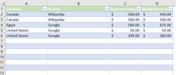
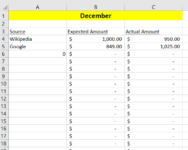
I have a workbook with thirteen sheets, named January through December, with the last sheet being named Totals. In each of the first twelve sheets, I have tables (with headers), named the same as the tab that they are on. Example, Tab named January with a table named January. All thirteen forms have the same formatting for tables, same number of columns and row, with the same header values. On sheets January to December, the table starts in A1. On the Totals sheet, the table starts in C1. I have a drop down validation list in cell A1 of the Totals sheets with a list of the other sheet names. I would like a formula that will pull a sum of the data from each respective table, based on the value in cell A1 from the validation list. There are no formulas on the first twelve sheets, but I am currently using the following formulas (which need to be fixed) on the Totals sheet.
Current Formulas:
Cell A4 =IFERROR(INDEX(December[[Source ]], MATCH(0,COUNTIF(A$1:$E3,December[[Source ]]), 0)),"")
Cell B4 =SUMIF(December[[Source ]],A4,December[Expected Amount])
Cell B5 =SUMIF(December[[Source ]],A4,December[Actual Amount])

So my question..... How do I use cell A1 value within a formula to get the information that I need? I have attached two photos for reference. The first is of sheet December, the second is of sheet Totals.
 

Attachments

  • December.png
    December.png
    17.5 KB · Views: 20
  • Totals.png
    Totals.png
    18 KB · Views: 21

Excel Facts

Using Function Arguments with nested formulas
If writing INDEX in Func. Arguments, type MATCH(. Use the mouse to click inside MATCH in the formula bar. Dialog switches to MATCH.
Hi Wryan_Garner4,

With your 365 you'll have a better option to retrieve the distinct source entries but with my Excel 2016 I'll use AGGREGATE.

I believe this does what you want.


wryan_garner4.xlsx
ABCD
1LocationSourceExpected AmountActual Amount
2CanadaWikipedia500450
3CanadaWikipedia500500
4EgyptGoogle500675
5United StatesGoogle5050
6United StatesGoogle299300
7
8
9
10
11
December


wryan_garner4.xlsx
ABC
1December
2
3SourceExpected AmountActual Amount
4Wikipedia$ 1,000.00$ 950.00
5Google$ 849.00$ 1,025.00
6 
7 
Totals
Cell Formulas
RangeFormula
A4:A7A4=IFERROR(INDEX(INDIRECT($A$1&"["&A$3&"]"),AGGREGATE(15,6,ROW(INDIRECT($A$1&"["&A$3&"]"))-1/(ISNA(MATCH(INDIRECT($A$1&"["&A$3&"]"),$A$3:$A3,0))),1))&"","")
B4:C7B4=IF($A4="","",SUMIF(INDIRECT($A$1&"["&$A$3&"]"),$A4,INDIRECT($A$1&"["&B$3&"]")))
 
Upvote 0
Another option for xl365
+Fluff 1.xlsm
ABC
1December
2
3SourceExpected AmountActual Amount
4Wikipedia1000950
5Google8491025
Main
Cell Formulas
RangeFormula
A4:A5A4=LET(tbl,INDIRECT(A1&"["&A3&"]"),UNIQUE(FILTER(tbl,tbl<>"")))
B4:C5B4=SUMIFS(INDIRECT($A$1&"["&B$3&"]"),INDIRECT($A$1&"["&$A$3&"]"),$A4#)
Dynamic array formulas.
Thank you. This has worked well for me. I am now trying to add a couple columns to the right that will pull that same Source list from all sheets, remove duplicates, then get a sum of all of the Expected Amounts and Actual Amounts. I have tried adjusting the formula to search all sheets, but haven't had good luck. Any thoughts?
 
Upvote 0

Forum statistics

Threads
1,214,832
Messages
6,121,853
Members
449,051
Latest member
excelquestion515

We've detected that you are using an adblocker.

We have a great community of people providing Excel help here, but the hosting costs are enormous. You can help keep this site running by allowing ads on MrExcel.com.
Allow Ads at MrExcel

Which adblocker are you using?

Disable AdBlock

Follow these easy steps to disable AdBlock

1)Click on the icon in the browser’s toolbar.
2)Click on the icon in the browser’s toolbar.
2)Click on the "Pause on this site" option.
Go back

Disable AdBlock Plus

Follow these easy steps to disable AdBlock Plus

1)Click on the icon in the browser’s toolbar.
2)Click on the toggle to disable it for "mrexcel.com".
Go back

Disable uBlock Origin

Follow these easy steps to disable uBlock Origin

1)Click on the icon in the browser’s toolbar.
2)Click on the "Power" button.
3)Click on the "Refresh" button.
Go back

Disable uBlock

Follow these easy steps to disable uBlock

1)Click on the icon in the browser’s toolbar.
2)Click on the "Power" button.
3)Click on the "Refresh" button.
Go back
Back
Top