In my example, E has the rankings for column B, F has the rankings for column C, and G has the rankings for column D. If you only want the column B rankings, just remove the formulas from columns F and G.
In my example, E has the rankings for column B, F has the rankings for column C, and G has the rankings for column D. If you only want the column B rankings, just remove the formulas from columns F and G.
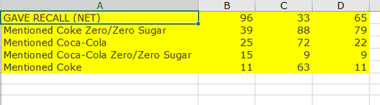
Can you show an example of what you're looking for? If you use C and D columns as secondary and 3rd parameters, they would only come into play if column B has ties, which is not the case in your example. Please make an example with some numbers, and show the expected results and explain how you got them.
We have a great community of people providing Excel help here, but the hosting costs are enormous. You can help keep this site running by allowing ads on MrExcel.com.
Allow Ads at MrExcel
Which adblocker are you using?
Disable AdBlock
Follow these easy steps to disable AdBlock
1)Click on the icon in the browser’s toolbar. 2)Click on the icon in the browser’s toolbar. 2)Click on the "Pause on this site" option.
Go back
Disable AdBlock Plus
Follow these easy steps to disable AdBlock Plus
1)Click on the icon in the browser’s toolbar. 2)Click on the toggle to disable it for "mrexcel.com".
Go back
Disable uBlock Origin
Follow these easy steps to disable uBlock Origin
1)Click on the icon in the browser’s toolbar. 2)Click on the "Power" button. 3)Click on the "Refresh" button.
Go back
Disable uBlock
Follow these easy steps to disable uBlock
1)Click on the icon in the browser’s toolbar. 2)Click on the "Power" button. 3)Click on the "Refresh" button.