VBA Check for multiple cell values and copy the cell in column A

[Goldyyyy]

Hello!

So I have this code that checks for the values in column "L" in this case it's 25. But I want to change this code so that it actually checks for the value in column "J" and "K". So for example right now if we get the value 25, it copy's the cell in column A and paste's it in different sheet in cell "G1".

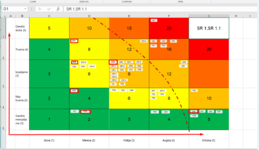
What I want to accomplish is to check for the values in the column "J" and "K" and if for example both of the values are "5" then again copy the cell value in Column "A" and paste it the other sheet in "G1" because when you multiple 5*5 it's 25, but if the values are for example "J" is 5 and "K" is 4 then it's 20, so it should paste the cell value from column "A" into the other sheet in cell "F1". But again if the value in "J" is 4 and in "K" it's 5 then also 20, but now it should actually paste the value now not in "F1"but "G2" a It's like a multiplier and according to the values of these both numbers I have to put them in the correct place in the map that you can see below. I guess it will be a lot of if else statements or something, because it has to check all the possible values which are in column "J" 1-5 and in "K" also 1-5.

THIS IS THE CODE THAT I HAVE RIGHT NOW.

Public Sub FindingValues()
    Dim val As Integer, result As String, firstAddress As String
    Dim a As Range

    val = 25
    Set a = Sheets("riskuregistrs").Range("L:L").Find(val, LookIn:=xlValues, Lookat:=xlWhole, MatchCase:=False)

    If Not a Is Nothing Then
        firstAddress = a.Address

        Do
            If Len(result) > 0 Then
                result = result & "," & a.Offset(0, -11).Text
            Else
                result = a.Offset(0, -11).Text
            End If

            Set a = Cells.FindNext(a)
        Loop While Not a Is Nothing And a.Address <> firstAddress
    End If

    Sheets("Riskukarte").Range("G1").Value = result
End Sub

These are the excel sheet's where I have to take the value from and the third image is the map where the values from column "A" from the first sheet should be pasted. As you can see in cell "G1" it pasted all the cell values that had number 25 in column "L".







I will appreciate any help I could get. Thank you so much in advance! If there is any other questions regarding this, please - ask.

 

[Anthony47]

Can you share a sample workbook, so we have not to waste time in creating a suitable test bed? Also, in your destination map, can you specify wether the column position depends on value of column J and the row position on the value of column K, or viceversa? (in your examples you use 5*5 and 4*4 that don't clarify this aspect)
To share a workbook you have to upload your file to a filesharing service (for example filedropper.com) and the publish the download linf the file will be assigned. Remove confidential information before sharing

Bye

 

[Goldyyyy]

Can you share a sample workbook, so we have not to waste time in creating a suitable test bed? Also, in your destination map, can you specify wether the column position depends on value of column J and the row position on the value of column K, or viceversa? (in your examples you use 5*5 and 4*4 that don't clarify this aspect)
To share a workbook you have to upload your file to a filesharing service (for example filedropper.com) and the publish the download linf the file will be assigned. Remove confidential information before sharing

Bye

Hi Anthony! Thank you for your reply! Destination map is inside "Riskukarte" and yes the value does depend. As you can see in the map for example if the value in column "J" is 3 and in "K" is 4 then the total would be 12 and the position would have to be "F3", but if "J" is 4 and "K" is 3 then the position would be "E2".

This is the link to the file - https://failiem.lv/u/pumrv8j2

Also when running the macro on your computer, make sure that the sheet with name "riskuregistrs" is open, because if you run the code while being in the "Riskukarte" it gives an error. Than

 

[Goldyyyy]

I just forgot to mention that inside "Riskukarte" you should see it like a multiplier table if that makes sense. Y is from 1-5 and X is from 1-5. Check image below, it will make sense if my answer doesn't.

 

[Anthony47]

My best guess:

Sub RiskMap()
Dim LastA As Long, oArr(1 To 5, 1 To 5), wArr
Dim sSh As Worksheet, oSh As Worksheet, I As Long
Dim xCol As String, xNum As Long, yCol As String, yNum As Long

Set sSh = Sheets("riskuregistrs")       '<<<
Set oSh = Sheets("Riskukarte")          '<<<
'
xCol = "K"                              '<<<
yCol = "J"                              '<<<
'
xNum = Cells(1, xCol).Column
yNum = Cells(1, yCol).Column
LastA = sSh.Cells(Rows.Count, 1).End(xlUp).Row
wArr = sSh.Cells(1, 1).Resize(LastA, 13).Value
For I = 1 To UBound(wArr)
    If wArr(I, xNum) > 0 And wArr(I, xNum) < 6 And wArr(I, yNum) > 0 And wArr(I, yNum) < 6 Then
        If Len(oArr(6 - wArr(I, yNum), wArr(I, xNum))) = 0 Then
            oArr(6 - wArr(I, yNum), wArr(I, xNum)) = wArr(I, 1)
        Else
            oArr(6 - wArr(I, yNum), wArr(I, xNum)) = oArr(6 - wArr(I, yNum), wArr(I, xNum)) & ", " & wArr(I, 1)
        End If
    End If
Next I
oSh.Range("C1").Resize(5, 5).Value = oArr
MsgBox ("Done...")
End Sub

Bye

 

[Goldyyyy]

Anthony! Wow! I'm amazed! You're a legend! It works as intended! Thank you so much!

Anthony I have one more question. Is it possible to make the "A" column like small textboxes like in the image below?

I found some code that creates automatically the texbox, but it doesn't seem to fit this purpose. I am very new to VBA so I don't know how all this works, maybe it is possible to somehow implement this texbox code inside yours.

Sub AddTextBox()
Dim ws As Worksheet
Dim oTB As Object
Set ws = Worksheets("Sheet2")
   Set oTB = ws.OLEObjects.Add(ClassType:="Forms.TextBox.1")
    With oTB
    .Name = "MyTB"
    .LinkedCell = "$A$2"
    .Left = ws.Range("B2").Left
    .Top = ws.Range("B2").Left
    .Width = ws.Range("B2").Width
    .Height = ws.Range("B2").Height
    .Object.BackColor = RGB(204, 204, 255)
    .Object.ForeColor = RGB(0, 0, 255)
    .Object.Text = "Hello"
    End With

End Sub

 

[Anthony47]

Which is the reason for having those "textboxes"? Aesthetic? Visibility? Ease of access? Or...??

 

[Goldyyyy]

Which is the reason for having those "textboxes"? Aesthetic? Visibility? Ease of access? Or...??

It is Visibility. Basically they should be as small as they can be, the image that I uploaded earlier is like an example, but how to do it, no idea. Basically in my company each week there are meeting where you need to show this RiskMap, because the values change and we have to show these changes and for now we move texboxes manually, so we’re looking to automate this process.

 

[Anthony47]

Just for fun I tried adding shapes to the cells.
For this I started from the macro already prepared, and created two additional macros that are "called" by the main macro to adding and formatting the shapes.
The modified main macro:

Sub RiskMap22()
Dim LastA As Long, OArr(1 To 5, 1 To 5), wArr
Dim sSh As Worksheet, oSh As Worksheet, I As Long
Dim xCol As String, xNum As Long, yCol As String, yNum As Long

Set sSh = Sheets("riskuregistrs")       '<<<
Set oSh = Sheets("Riskukarte")          '<<<
'
xCol = "K"                              '<<<
yCol = "J"                              '<<<
'
xNum = Cells(1, xCol).Column
yNum = Cells(1, yCol).Column
LastA = sSh.Cells(Rows.Count, 1).End(xlUp).Row
wArr = sSh.Cells(1, 1).Resize(LastA, 13).Value
For I = 1 To UBound(wArr)
    If wArr(I, xNum) > 0 And wArr(I, xNum) < 6 And wArr(I, yNum) > 0 And wArr(I, yNum) < 6 Then
        If Len(OArr(6 - wArr(I, yNum), wArr(I, xNum))) = 0 Then
            OArr(6 - wArr(I, yNum), wArr(I, xNum)) = wArr(I, 1)
        Else
            OArr(6 - wArr(I, yNum), wArr(I, xNum)) = OArr(6 - wArr(I, yNum), wArr(I, xNum)) & ", " & wArr(I, 1)
        End If
    End If
Next I
'Modified area >>>
'Select Output sheet and populate:
oSh.Select
oSh.Range("C1").Resize(5, 5).Value = OArr   'Cell values
Call TBPos(OArr)                            'Set Shapes
MsgBox ("Done...")
'Autozoom the output table:
Range("C1").Resize(5, 5).Select
ActiveWindow.Zoom = True
Range("C1").Select
End Sub

The additional code:

'Insert shapes
Dim cRisk As String, qtArr(1 To 5, 1 To 5) As Integer
Dim fPos As Integer, shW As Integer, shH As Integer
Dim mySplit, fCnt As Integer, cfCnt As Integer, ifCnt As Integer
Dim Top0 As Integer, Left0 As Integer, K As Integer, J As Integer
'
'Calculate Shapes size:
shW = (ActiveSheet.Range("C1").Width - 2 * 2) / 4
shH = (ActiveSheet.Range("C1").Height - 2 * 2) / 7
'Remove existing shapes:
With ActiveSheet
    shcnt = .Shapes.Count
    For I = shcnt To 1 Step -1
        If .Shapes(I).Type = msoAutoShape Then
            .Shapes(I).Delete
        Else
            .Shapes(I).Top = (shcnt - I) * shH + 10
            .Shapes(I).Left = Range("S1").Left - I
        End If
    Next I
    DoEvents: DoEvents
    'Calculate highest shapes number:
    For J = 1 To UBound(OArr)
        For K = 1 To UBound(OArr, 2)
            cfCnt = (Len(OArr(J, K)) - Len(Replace(OArr(J, K), ",", "", , , vbTextCompare)))
            If cfCnt > fCnt Then fCnt = cfCnt
        Next K
    Next J
    'Examine oArr content and insert requested shapes in position:
    For J = 1 To UBound(OArr)
        For K = 1 To UBound(OArr, 2)
            Range("C1").Cells(J, K).Select      'debug only
            'Rows to insert:
            cfCnt = 1 + Int((Len(OArr(J, K)) - Len(Replace(OArr(J, K), ",", "", , , vbTextCompare))) / 4)
            'Calculate top spacer:
            Top0 = (Range("C1").Cells(J, K).Height - cfCnt * shH) / 2
            Left0 = 0                           'Reset left spacer
            'create X elements for the cell:
            mySplit = Split(OArr(J, K), ", ", , vbTextCompare)
            'Examine each element:
            For I = 0 To UBound(mySplit)
                If (cfCnt - Int(I / 4)) = 1 Then    'on last line, calculate left spacer
                    If Left0 = 0 Then Left0 = (Range("C1").Cells(J, K).Width - (UBound(mySplit) - I + 1) * shW) / 2
                Else
                    Left0 = 0
                End If
                fTop = 2 + .Range("C1").Cells(J, K).Top + Int(I / 4) * (shH) + Top0         'Shape top
                fLeft = 2 + .Range("C1").Cells(J, K).Left + (I Mod 4) * (shW) + Left0       'Shape left
                Call AddShape(fTop, fLeft, shW - 2, shH - 2, mySplit(I))                    'Create and format the shape
            Next I
        Next K
    Next J
End With
Range("C1").Select
End Sub



Sub AddShape(ByVal fTop As Integer, ByVal fLeft As Integer, _
   ByVal fWdh As Integer, ByVal fHht As Integer, ByVal ITxt As String)
'Create and format shapes
    ActiveSheet.Shapes.AddShape(msoShapeRoundedRectangle, fLeft, _
        fTop, fWdh, fHht).Select
    With Selection.ShapeRange(1).TextFrame2
        .TextRange.Characters.Text = ITxt
        .TextRange.Characters.Font.Size = 8
        .TextRange.Characters.Font.Bold = msoTrue
        .VerticalAnchor = msoAnchorMiddle
        .MarginLeft = 2
        .MarginRight = 2
        .MarginTop = 2
        .MarginBottom = 2
        .WordWrap = msoFalse
    End With
    With Selection.ShapeRange(1).TextFrame2.TextRange.Characters. _
        ParagraphFormat
        .FirstLineIndent = 0
        .Alignment = msoAlignCenter
    End With
    Selection.ShapeRange.ShapeStyle = msoShapeStylePreset7
    With Selection.ShapeRange.Line
        .Visible = msoTrue
        .ForeColor.ObjectThemeColor = msoThemeColorText1
        .ForeColor.TintAndShade = 0
        .ForeColor.Brightness = 0
        .Transparency = 0
        .Visible = msoTrue
        .Weight = 0.5
    End With
End Sub

It is important that the rows and columns of output table have the same width and height, or the position of the shapes would be erratic.
Note that, at the moment, the cells are stll compiled as they were with the previous macro. This is mainly for cheching that the shapes reflect the calculated Risk Id. If cells are formatted for "wrap text", "horizontal central alignement" and "vertical central alignment" probably the cells values are hidden by the shapes; in this case doublecliccking the cell will make the content fully visible.

Try...

 

[Goldyyyy]

.