VBA code - Calculated weighted average in pivot table without 0 values

[NieuwNat]

Dear all,

I hope you can help me with the following issue, because I'm completely new with VBA code and I'm learning at the moment.

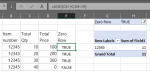
I'm creating a Pivot table in Sheet B based on input from Sheet A. Let's assume I've the following lines.

Item number	Total Qty	Total Price
12345	10	100
12345	20	200
12345	30	360
12345	40	0

I have the following code now:

This is for the calculation of the field:
ActiveSheet.PivotTables("ForecastPivotTable").CalculatedFields.Add Name:="WAVG Forecast Price", _
Formula:="=IFERROR(Calculated Finance Forecast/Calculated Sales Forecast,0)"

This is to show the field in the Pivot Table which is created with VBA Code:
With ActiveSheet.PivotTables("ForecastPivotTable").PivotFields("WAVG Forecast Price")
.Orientation = xlDataField
.Function = xlSum
.NumberFormat = "0.00"

The result now is that the WAVG Forecast Price = 6,6. But this is incorrect. I would like to leave out all the lines for the item number with a 0 value in the Total Price and/or in the Total Qty. The result should be (100+200+360)=660 divided by (10+20+30)=60 = 660/60=11.

I hope somebody can help me out to find the correct Formula:= for this. I've tried several things I found on Google, like AVERAGEIFS or SUMPRODUCT, but nothing worked. Probably I made some mistakes.

Thank you very much for your help.

 

[G12]

Hi.
An alternative option for you. Why not flag the zero rows in your data source (Where E has the formula =AND(C4<>0,D4<>0)). Then you can use your calculated field (price/qty) in the pivot

Would that work for you?
Let me know
G12

 

[NieuwNat]

Hi.
An alternative option for you. Why not flag the zero rows in your data source (Where E has the formula =AND(C4<>0,D4<>0)). Then you can use your calculated field (price/qty) in the pivot

View attachment 8658

Would that work for you?
Let me know
G12

Hi,

Thank you for your quick response. Unfortunately this will not work for me. I've a lot of other data on Sheet A which I also need for my Pivot table to create. By filtering this out, it will become a problem for my other data as well. I only need to exclude the values from Total Price and Total Quantity, without filtering the other data. I hope you have a solution for this to. Thank you.

 

[G12]

Hi.
Can you give me more on the data source? The table you've shown really is the results of the pivot, right? But your weighted average cost will be the running sum until the last result (in your case excluding 0 values for cost or quantity). So when you summarize the data, you'll always be summing these fields unless you can identify a way to exclude them from the pivot table.

If I was doing a running weighted average on the data source, I'd use SUMIFS to have the running weighted average excluding zeros. But I'm not following the intent to pull this in the pivot when you have 5 results rows with the same item number.

=SUMIFS(D$3:D3,B$3:B3,B3,C$3:C3,"<>0")/IF(SUMIFS(C$3:C3,B$3:B3,B3,D$3:D3,"<>0")=0,1,SUMIFS(C$3:C3,B$3:B3,B3,D$3:D3,"<>0"))

HTH
G12

 

[NieuwNat]

Hi.
Can you give me more on the data source? The table you've shown really is the results of the pivot, right? But your weighted average cost will be the running sum until the last result (in your case excluding 0 values for cost or quantity). So when you summarize the data, you'll always be summing these fields unless you can identify a way to exclude them from the pivot table.

If I was doing a running weighted average on the data source, I'd use SUMIFS to have the running weighted average excluding zeros. But I'm not following the intent to pull this in the pivot when you have 5 results rows with the same item number.

=SUMIFS(D$3:D3,B$3:B3,B3,C$3:C3,"<>0")/IF(SUMIFS(C$3:C3,B$3:B3,B3,D$3:D3,"<>0")=0,1,SUMIFS(C$3:C3,B$3:B3,B3,D$3:D3,"<>0"))

HTH
G12

View attachment 8665

Hi,

No, the data in Sheet A is the base data I use to create a pivot table in Sheet B. The figures I gave were only a small part of the row in Sheet A.

In Sheet A I have a lot of lines with also columns like Period, Sales Channel, Line of Business, Total Qty, Total Price and many others. One Item Number can be used in different Sales Channels.

In the pivot table I summarize all data from Sheet A on Item level (without Sales Channels) and Period. Then I need the total of the Quantity and I need an weighted average on the Price, but excluding the lines where there is a 0 value for Total Qty or Total Price.

 

[NieuwNat]

Hi,

No, the data in Sheet A is the base data I use to create a pivot table in Sheet B. The figures I gave were only a small part of the row in Sheet A.

In Sheet A I have a lot of lines with also columns like Period, Sales Channel, Line of Business, Total Qty, Total Price and many others. One Item Number can be used in different Sales Channels.

In the pivot table I summarize all data from Sheet A on Item level (without Sales Channels) and Period. Then I need the total of the Quantity and I need an weighted average on the Price, but excluding the lines where there is a 0 value for Total Qty or Total Price.

Also, in the pivot table I have a Total qty where I need the Total Qty, even if the Total Price is 0. So, it should only exlude the line when calculating the Total Price.

 

[NieuwNat]

Also, in the pivot table I have a Total qty where I need the Total Qty, even if the Total Price is 0. So, it should only exlude the line when calculating the Total Price.

And maybe also good to know, the data in Sheet A is dynamic. Therefore I create a pivot table in Sheet B with VBA code to summarize my data.

 

[G12]

I still think this is a fix with the data source. As a last attempt, perhaps you can add adjusted price & quantities columns to the data source. Then in your pivot, create a calculated field which calculates the adjusted weighted average.

Best of luck

 

[NieuwNat]

I still think this is a fix with the data source. As a last attempt, perhaps you can add adjusted price & quantities columns to the data source. Then in your pivot, create a calculated field which calculates the adjusted weighted average.

View attachment 8671

Best of luck

Thank you very much. This is indeed a good workaround which I can use and didn't thought of. I was hoping to solve it with a formula, but this will also work for me. Thank you very much for your help today! It's much appreciated.