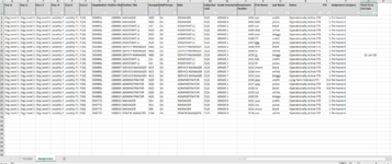
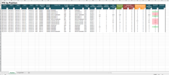
VBA code to split worksheet with multiple sheets

[shell2133]

Hello everyone. I would like to split a worksheet which has two sheets called "Position and "Assignment" at each change in column E, "Org L5", on both tabs, so create a new sheet with a position and assignment tab for each of the different Org L5s, preserving the headers and formulas etc. The headers on the Position tab are in A1:Y3, on the Assignment tab they're in A1:U1. I want to name the new sheets as per column E, the Org L5 name. I've done similar for one tab before but not two and I'm also struggling with the header on the first tab with it being in multiple rows. Would anyone know a code for this please? Thanks!

 

[mumps]

When you add a workbook, the default number of sheets is 3. If you are only getting one sheet, you may have to change the settings in Excel. You can do that by clicking FILE...OPTIONS...GENERAL and change the number in the "Include this many sheets" box.
This version of the macro should work:

Sub CreateWorkbooks()
    Application.ScreenUpdating = False
    Dim posWS As Worksheet, assWS As Worksheet, v As Variant, dic As Object, i As Long, WB As Workbook
    Set WB = ThisWorkbook
    Set posWS = WB.Sheets("Position")
    Set assWS = WB.Sheets("Assignment")
    Set dic = CreateObject("Scripting.Dictionary")
    With posWS
        v = .Range("E4", .Range("E" & .Rows.Count).End(xlUp)).Value
        For i = LBound(v) To UBound(v)
            If Not dic.exists(v(i, 1)) Then
                dic.Add v(i, 1), Nothing
                .Range("A1").CurrentRegion.AutoFilter 5, v(i, 1)
                .AutoFilter.Range.Offset(1).Copy
                Workbooks.Add
                Range("A4").PasteSpecial
                ActiveSheet.Name = "Position"
                .Range("A1").AutoFilter
                .Range("A1:Y3").Copy Range("A1")
                Columns.AutoFit
                Sheets.Add(After:=Sheets(Sheets.Count)).Name = "Assignment"
                With assWS
                    .Range("A1").CurrentRegion.AutoFilter 5, v(i, 1)
                    .AutoFilter.Range.Copy
                    Range("A1").PasteSpecial
                End With
                With ActiveWorkbook
                    Application.DisplayAlerts = False
                    .SaveAs Filename:="C:\Users\shell\Documents\" & v(i, 1), FileFormat:=51
                    .Close False
                    Application.DisplayAlerts = True
                End With
            End If
        Next i
    End With
    assWS.Range("A1").AutoFilter
    Application.ScreenUpdating = True
End Sub

 

[shell2133]

That's very nearly perfect! The formula in column P on the new Position tab is still referring to the original Staff List sheet - e.g. in cell P4 its "=COUNTIFS('[STAFF LIST.xlsx]Assignment'!$H$2:$H$25,$H4)". Is there a way to change that so it just looks at the Assignment tab of the newly created sheet? So reads just "=COUNTIFS('Assignment'!$H$2:$H$25,$H4)". Is it also possible to automatically hide the new sheets Sheet2 and Sheet3 as they're just blank? Thank you for your patience with this

 

[mumps]

Try:

Sub CreateWorkbooks()
    Application.ScreenUpdating = False
    Dim posWS As Worksheet, assWS As Worksheet, v As Variant, dic As Object, i As Long, WB As Workbook
    Set WB = ThisWorkbook
    Set posWS = WB.Sheets("Position")
    Set assWS = WB.Sheets("Assignment")
    Set dic = CreateObject("Scripting.Dictionary")
    With posWS
        v = .Range("E4", .Range("E" & .Rows.Count).End(xlUp)).Value
        For i = LBound(v) To UBound(v)
            If Not dic.exists(v(i, 1)) Then
                dic.Add v(i, 1), Nothing
                .Range("A1").CurrentRegion.AutoFilter 5, v(i, 1)
                .AutoFilter.Range.Offset(1).Copy
                Workbooks.Add
                Range("A4").PasteSpecial
                ActiveSheet.Name = "Position"
                .Range("A1").AutoFilter
                .Range("A1:Y3").Copy Range("A1")
                Columns.AutoFit
                Sheets.Add(After:=Sheets(Sheets.Count)).Name = "Assignment"
                With assWS
                    .Range("A1").CurrentRegion.AutoFilter 5, v(i, 1)
                    .AutoFilter.Range.Copy
                    Range("A1").PasteSpecial
                    Sheets("Position").Range("P4", Sheets("Position").Range("P" & Rows.Count).End(xlUp)).Formula = "=COUNTIFS(Assignment!$H$2:$H$" & assWS.Range("P" & Rows.Count).End(xlUp).Row & ",$H4)"
                    .Range("A1").AutoFilter
                    Columns.AutoFit
                End With
                With ActiveWorkbook
                    Application.DisplayAlerts = False
                    .Sheets("Sheet2").Delete
                    .Sheets("Sheet3").Delete
                    .SaveAs Filename:="C:\Users\shell\Documents\" & v(i, 1), FileFormat:=51
                    .Close False
                    Application.DisplayAlerts = True
                End With
            End If
        Next i
    End With
    Application.ScreenUpdating = True
End Sub

 

[shell2133]

I think that's it! Thanks ever so much for all your help

 

[mumps]

My pleasure.