VBA or formula to transpose/re-arranging data in columns

[rozek]

Hello. Appreciate any help on this transpose/re-arranging of columns. What I wanted to achieved is straight forward but seems difficult to do.

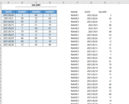
I wanted to re arrange this dataset below:

Book1
	A	B	C	D
1		SALARY
2	DATE	NAME1	NAME2	NAME3
3	1/1/2021	10	1	100
4	2/1/2021	20	2	200
5	3/1/2021	30	3	300
6	4/1/2021	40	4	400
7	5/1/2021	50	5	500
8	6/1/2021	60	6	600
9	7/1/2021	70	7	700
10	8/1/2021	80	8	800
11	9/1/2021	90	9	900
12	10/1/2021	100	10	1000
Sheet1 (2)

To be in this arrangement

Book1
	A	B	C
1	NAME	DATE	SALARY
2	NAME1	1/1/2021	10
3	NAME1	2/1/2021	20
4	NAME1	3/1/2021	30
5	NAME1	4/1/2021	40
6	NAME1	5/1/2021	50
7	NAME1	6/1/2021	60
8	NAME1	7/1/2021	70
9	NAME1	8/1/2021	80
10	NAME1	9/1/2021	90
11	NAME1	10/1/2021	100
12	NAME2	1/1/2021	1
13	NAME2	2/1/2021	2
14	NAME2	3/1/2021	3
15	NAME2	4/1/2021	4
16	NAME2	5/1/2021	5
17	NAME2	6/1/2021	6
18	NAME2	7/1/2021	7
19	NAME2	8/1/2021	8
20	NAME2	9/1/2021	9
21	NAME2	10/1/2021	10
22	NAME3	1/1/2021	100
23	NAME3	2/1/2021	200
24	NAME3	3/1/2021	300
25	NAME3	4/1/2021	400
26	NAME3	5/1/2021	500
27	NAME3	6/1/2021	600
28	NAME3	7/1/2021	700
29	NAME3	8/1/2021	800
30	NAME3	9/1/2021	900
31	NAME3	10/1/2021	1000
Sheet1 (2)

Any help is much appreciated. Thank you.

 

[Hileolane]

You can consider to use powerquery to complete it with a few clicks. It will be quite easy.

 

[rozek]

Thank you for the reply. I prefer if this could be done using VBA since need to combine with other automation.

 

[Hileolane]

As I don't know the target cells range to display the final data, I can't write VBA codes correspondingly but I did make it happen.

Sub Rearrange()
Application.ScreenUpdating = False

Dim rng As Range

For Each rng In Selection
        Range("F10000").End(3).Offset(1).Value = Cells(3, rng.Column).Text
        Range("G10000").End(3).Offset(1).Value = Cells(rng.Row, 1).Text
        Range("H10000").End(3).Offset(1).Value = rng.Value
Next
Application.ScreenUpdating = True

End Sub

Step 1 Make sure the layout of the original data.
Step 2 Select the salary area, i.e. B4:D13 in my case
Step 3 Run the vba macro

 

[Peter_SSs]

VBA or formula to transpose/re-arranging data in columns

Here is a formula approach. You only need to enter this formula in the top-left result cell and the results should automatically spill to the required rows and columns.

21 08 24.xlsm
	A	B	C	D	E	F	G	H
1		SALARY
2	DATE	NAME1	NAME2	NAME3		NAME	DATE	SALARY
3	1/01/2021	10	1	100		NAME1	1/01/2021	10
4	2/01/2021	20	2	200		NAME1	2/01/2021	20
5	3/01/2021	30	3	300		NAME1	3/01/2021	30
6	4/01/2021	40	4	400		NAME1	4/01/2021	40
7	5/01/2021	50	5	500		NAME1	5/01/2021	50
8	6/01/2021	60	6	600		NAME1	6/01/2021	60
9	7/01/2021	70	7	700		NAME1	7/01/2021	70
10	8/01/2021	80	8	800		NAME1	8/01/2021	80
11	9/01/2021	90	9	900		NAME1	9/01/2021	90
12	10/01/2021	100	10	1000		NAME1	10/01/2021	100
13						NAME2	1/01/2021	1
14						NAME2	2/01/2021	2
15						NAME2	3/01/2021	3
16						NAME2	4/01/2021	4
17						NAME2	5/01/2021	5
18						NAME2	6/01/2021	6
19						NAME2	7/01/2021	7
20						NAME2	8/01/2021	8
21						NAME2	9/01/2021	9
22						NAME2	10/01/2021	10
23						NAME3	1/01/2021	100
24						NAME3	2/01/2021	200
25						NAME3	3/01/2021	300
26						NAME3	4/01/2021	400
27						NAME3	5/01/2021	500
28						NAME3	6/01/2021	600
29						NAME3	7/01/2021	700
30						NAME3	8/01/2021	800
31						NAME3	9/01/2021	900
32						NAME3	10/01/2021	1000
Rearrange

Cell Formulas
Range	Formula
F3:H32	F3	=LET(rws,ROWS(A3:A12),cols,COLUMNS(B2:D2),c_1,INDEX(B2:D2,INT(SEQUENCE(rws*cols,,rws)/rws)),c_2,INDEX(A3:A12,MOD(SEQUENCE(rws*cols,,0),rws)+1),CHOOSE({1,2,3},c_1,c_2,INDEX(B3:D12,MATCH(c_2,A3:A12,0),MATCH(c_1,B2:D2,0))))
Dynamic array formulas.

 

[Hileolane]

I use INDEX to get the answer for you too

ReArrange.xlsx
	A	B	C	D	E	F	G	H	I	J
1		SALARY
2									先做这个 利用index是引用的属性
3	DATE	NAME1	NAME2	NAME3			NAME	DATE	SALARY
4	2021/8/26	3	42	5			NAME1	2021/8/26	3
5	2021/9/3	90	72	64			NAME1	2021/9/3	90
6	2021/8/26	43	37	12			NAME1	2021/8/26	43
7	2021/8/15	37	51	19			NAME1	2021/8/15	37
8	2021/8/22	7	54	41			NAME1	2021/8/22	7
9	2021/8/14	79	70	36			NAME1	2021/8/14	79
10	2021/8/23	72	6	31			NAME1	2021/8/23	72
11	2021/8/29	46	85	72			NAME1	2021/8/29	46
12	2021/8/28	60	15	14			NAME1	2021/8/28	60
13	2021/8/20	33	29	48			NAME1	2021/8/20	33
14							NAME2	2021/8/26	42
15							NAME2	2021/9/3	72
16							NAME2	2021/8/26	37
17							NAME2	2021/8/15	51
18							NAME2	2021/8/22	54
19							NAME2	2021/8/14	70
20							NAME2	2021/8/23	6
21							NAME2	2021/8/29	85
22							NAME2	2021/8/28	15
23							NAME2	2021/8/20	29
24							NAME3	2021/8/26	5
25							NAME3	2021/9/3	64
26							NAME3	2021/8/26	12
27							NAME3	2021/8/15	19
28							NAME3	2021/8/22	41
29							NAME3	2021/8/14	36
30							NAME3	2021/8/23	31
31							NAME3	2021/8/29	72
32							NAME3	2021/8/28	14
33							NAME3	2021/8/20	48
数据逆透视

Cell Formulas
Range	Formula
G4:G33	G4	=INDEX($3:$3,,COLUMN(INDEX(INDEX($B$4:$D$13,,ROUNDUP(ROWS($E$4:E4)/ROWS($B$4:$B$13),0)),IF(MOD(ROWS($E$4:E4),ROWS($B$4:$B$13))=0,ROWS($B$4:$B$13),MOD(ROWS($E$4:E4),ROWS($B$4:$B$13))))))
H4:H33	H4	=INDEX(A:A,ROW(INDEX(INDEX($B$4:$D$13,,ROUNDUP(ROWS($E$4:E4)/ROWS($B$4:$B$13),0)),IF(MOD(ROWS($E$4:E4),ROWS($B$4:$B$13))=0,ROWS($B$4:$B$13),MOD(ROWS($E$4:E4),ROWS($B$4:$B$13))))))
I4:I33	I4	=INDEX(INDEX($B$4:$D$13,,ROUNDUP(ROWS($E$4:E4)/ROWS($B$4:$B$13),0)),IF(MOD(ROWS($E$4:E4),ROWS($B$4:$B$13))=0,ROWS($B$4:$B$13),MOD(ROWS($E$4:E4),ROWS($B$4:$B$13))))

 

[rozek]

Thank you Peter. Awesome formula. Just curious if its difficult to write this in VBA? Any help is appreciated for benefit of others as well.

 

[rozek]

I use INDEX to get the answer for you too

ReArrange.xlsx
	A	B	C	D	E	F	G	H	I	J
1		SALARY
2									先做这个 利用index是引用的属性
3	DATE	NAME1	NAME2	NAME3			NAME	DATE	SALARY
4	2021/8/26	3	42	5			NAME1	2021/8/26	3
5	2021/9/3	90	72	64			NAME1	2021/9/3	90
6	2021/8/26	43	37	12			NAME1	2021/8/26	43
7	2021/8/15	37	51	19			NAME1	2021/8/15	37
8	2021/8/22	7	54	41			NAME1	2021/8/22	7
9	2021/8/14	79	70	36			NAME1	2021/8/14	79
10	2021/8/23	72	6	31			NAME1	2021/8/23	72
11	2021/8/29	46	85	72			NAME1	2021/8/29	46
12	2021/8/28	60	15	14			NAME1	2021/8/28	60
13	2021/8/20	33	29	48			NAME1	2021/8/20	33
14							NAME2	2021/8/26	42
15							NAME2	2021/9/3	72
16							NAME2	2021/8/26	37
17							NAME2	2021/8/15	51
18							NAME2	2021/8/22	54
19							NAME2	2021/8/14	70
20							NAME2	2021/8/23	6
21							NAME2	2021/8/29	85
22							NAME2	2021/8/28	15
23							NAME2	2021/8/20	29
24							NAME3	2021/8/26	5
25							NAME3	2021/9/3	64
26							NAME3	2021/8/26	12
27							NAME3	2021/8/15	19
28							NAME3	2021/8/22	41
29							NAME3	2021/8/14	36
30							NAME3	2021/8/23	31
31							NAME3	2021/8/29	72
32							NAME3	2021/8/28	14
33							NAME3	2021/8/20	48
数据逆透视

Cell Formulas
Range	Formula
G4:G33	G4	=INDEX($3:$3,,COLUMN(INDEX(INDEX($B$4:$D$13,,ROUNDUP(ROWS($E$4:E4)/ROWS($B$4:$B$13),0)),IF(MOD(ROWS($E$4:E4),ROWS($B$4:$B$13))=0,ROWS($B$4:$B$13),MOD(ROWS($E$4:E4),ROWS($B$4:$B$13))))))
H4:H33	H4	=INDEX(A:A,ROW(INDEX(INDEX($B$4:$D$13,,ROUNDUP(ROWS($E$4:E4)/ROWS($B$4:$B$13),0)),IF(MOD(ROWS($E$4:E4),ROWS($B$4:$B$13))=0,ROWS($B$4:$B$13),MOD(ROWS($E$4:E4),ROWS($B$4:$B$13))))))
I4:I33	I4	=INDEX(INDEX($B$4:$D$13,,ROUNDUP(ROWS($E$4:E4)/ROWS($B$4:$B$13),0)),IF(MOD(ROWS($E$4:E4),ROWS($B$4:$B$13))=0,ROWS($B$4:$B$13),MOD(ROWS($E$4:E4),ROWS($B$4:$B$13))))

Thank you

Hileolane​

 

[Peter_SSs]

Just curious if its difficult to write this in VBA?

Should I assume

1. That there could be more or less than 10 rows of actual data?
2. That there could be more or less than 3 names in row 2?
3. That the 'DATE' heading will be in cell A2 of the active sheet?

 

[rozek]

Should I assume

1. That there could be more or less than 10 rows of actual data?
2. That there could be more or less than 3 names in row 2?
3. That the 'DATE' heading will be in cell A2 of the active sheet?

1. That there could be more or less than 10 rows of actual data? Since this is for number of days in a month. (can be 28/29, 30 or 31 days) equivalent to this much rows.
2. That there could be more or less than 3 names in row 2? Yes, it could be more but for example purposes, 3 names should be ok.
3. That the 'DATE' heading will be in cell A2 of the active sheet? Heading name is not compulsory but good to have at that cell. The arrangement of data is important.