VBA Self populate page name in formula

Edwardvanschothorst

New Member
Joined
Sep 20, 2021
Messages
14
Office Version
  1. 365
Platform
  1. Windows
First post here - I have been reading this forum for years, but this time I could not find what I am looking for so I am looking for a little help.

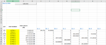
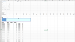
I am working on a worksheet that calculates part costs after I run after I optimize the cut lengths. I am using the 1dcutx add in to optimize my linear stock. (1DCutX - Length Cutting Optimization for Excel)
Once the stock is optimized it adds a range of worksheets starting at 1d_1 - 1d_xx depending on the different amount of layouts required for the job. Each of these sheets needs to have a formula added to distribute the waste length over the number of parts cut out of each length of material, and calculate the part cost based on material length. (part costs comes from my stock worksheet) Once these formula's are added I need to get the totals together in my parts worksheet so I can find the average cost of each part if it comes from various lengths. I have the script worked out to calculate this, but I have to write this code for each page that might exist. Is there a way to set this formula up so that it looks at all pages instead of writing this for each possible page? I could not get the mini uploader to work so I included screenshots of the parts list page, and the code for 1d_2, and 1d_3 below.

Private Sub two()
For i = 1 To Worksheets.Count
If Worksheets(i).Name = "1D_2" Then
Sheets("1D_2").Select
Range("e22") = "=roundup((b$7+2)/count(c$22:c$200)+c22+.055,3)"
Range("F22") = "=(VLOOKUP(A22,STOCK!$A$3:$C$20,3,FALSE)/VLOOKUP(A22,STOCK!$A$3:$C$20,2,FALSE)*E22)"
LastPopulatedRow = Range("A" & Rows.Count).End(xlUp).Row
Range("e22: " & "f" & LastPopulatedRow).FillDown
Sheets("Parts List").Select
Range("f14") = "=SUMPRODUCT(('1D_2'!$B$22:$B$140='Parts List'!$B14)*'1D_2'!$F$22:$F$140)*'1D_2'!$B$2"
LastPopulatedRow = Range("A" & Rows.Count).End(xlUp).Row
Range("f14: " & "f" & LastPopulatedRow).FillDown
MsgBox "1d_2 calculated"
End If
Next i
End Sub

Private Sub three()
For i = 1 To Worksheets.Count
If Worksheets(i).Name = "1D_3" Then
Sheets("1D_3").Select
Range("e22") = "=roundup((b$7+2)/count(c$22:c$200)+c22+.055,3)"
Range("F22") = "=(VLOOKUP(A22,STOCK!$A$3:$C$20,3,FALSE)/VLOOKUP(A22,STOCK!$A$3:$C$20,2,FALSE)*E22)"
LastPopulatedRow = Range("A" & Rows.Count).End(xlUp).Row
Range("e22: " & "f" & LastPopulatedRow).FillDown
Sheets("Parts List").Select
Range("g14") = "=SUMPRODUCT(('1D_3'!$B$22:$B$140='Parts List'!$B14)*'1D_3'!$F$22:$F$140)*'1D_3'!$B$2"
LastPopulatedRow = Range("A" & Rows.Count).End(xlUp).Row
Range("g14: " & "g" & LastPopulatedRow).FillDown
MsgBox "1d_3 calculated"
End If
Next i
End Sub
 

Attachments

  • parts list.PNG
    parts list.PNG
    36.9 KB · Views: 13
  • 1d_2.PNG
    1d_2.PNG
    55.5 KB · Views: 13
My apologies that was a mistake on my end. I missed a .name on the line above

Right now it is working however it is not poplulating the formula's on the 1d pages to give us the results in the cells below. In the columns for 1d1, and 1d2 I have an extra row as well.
linear stock production calc WIP 9.54.xlsm
ABCDEFGHIJKLM
13QTYPART NUMBERPART LENGTH (IN)1D_11D_21D_31D_41D_51D_61D_71D_81D_9
14375117733-12A2X2X.25000000000
150170212-13A2X2X.25000000000
166450141243-12A2x2x0.188000000000
17169157958-1138A2x2x0.188000000000
18132157959-1187A2x2x0.188000000000
1975157960-1210A2x2x0.188000000000
2075157961-139A2x2x0.188000000000
21113157962-16A2x2x0.188000000000
2200
Parts List
Cell Formulas
RangeFormula
E14:E22E14=SUMPRODUCT(('1D_1'!$B$22:$B$140='Parts List'!$B14)*'1D_1'!$F$22:$F$140)*'1D_1'!$B$2
F14:F22F14=SUMPRODUCT(('1D_2'!$B$22:$B$140='Parts List'!$B14)*'1D_2'!$F$22:$F$140)*'1D_2'!$B$2
G14:G21G14=SUMPRODUCT(('1D_3'!$B$22:$B$140='Parts List'!$B14)*'1D_3'!$F$22:$F$140)*'1D_3'!$B$2
H14:H21H14=SUMPRODUCT(('1D_4'!$B$22:$B$140='Parts List'!$B14)*'1D_4'!$F$22:$F$140)*'1D_4'!$B$2
I14:I21I14=SUMPRODUCT(('1D_5'!$B$22:$B$140='Parts List'!$B14)*'1D_5'!$F$22:$F$140)*'1D_5'!$B$2
J14:J21J14=SUMPRODUCT(('1D_6'!$B$22:$B$140='Parts List'!$B14)*'1D_6'!$F$22:$F$140)*'1D_6'!$B$2
K14:K21K14=SUMPRODUCT(('1D_7'!$B$22:$B$140='Parts List'!$B14)*'1D_7'!$F$22:$F$140)*'1D_7'!$B$2
L14:L21L14=SUMPRODUCT(('1D_8'!$B$22:$B$140='Parts List'!$B14)*'1D_8'!$F$22:$F$140)*'1D_8'!$B$2
M14:M21M14=SUMPRODUCT(('1D_9'!$B$22:$B$140='Parts List'!$B14)*'1D_9'!$F$22:$F$140)*'1D_9'!$B$2


linear stock production calc WIP 9.54.xlsm
ABCDEFGH
1Back to IndexPage:1D_3
2Qty:75
3Length:240
4Cost:3225
5Usage, %:95
6Waste, %5
7Offcut Length:12
8Material/Type:A2x2x0.188
9
10
11Cuts Info
12Cut No.1234
13Cut Location1188227239
14
15
16Qty:75
17
18
19
20
21Stock IDPart IDLengthLocationAdjusted lengthTTL Cost
22A2x2x0.188157959-11871
23A2x2x0.188157961-139188
24
1D_3
 
Upvote 0

Excel Facts

Bring active cell back into view
Start at A1 and select to A9999 while writing a formula, you can't see A1 anymore. Press Ctrl+Backspace to bring active cell into view.
Ok, so what should the formulas be in those ranges E14 :M21?
 
Upvote 0
We have a 99% solution - I added in the sheets(cursheetname).select, and it works other then on 1d sheets with a single line output. See excel range below script. I will keep working on this one.

VBA Code:
Sub AllSheetsV3()
'
    ColumnIncrementer = -1
'
    For i = 1 To Worksheets.Count
        cursheetname = Sheets(i).Name
        If Left(cursheetname, 3) = "1D_" And IsNumeric(Mid(cursheetname, 4, 1)) Then
            ColumnIncrementer = ColumnIncrementer + 1
Sheets(cursheetname).Select
            Range("e22") = "=roundup((b$7+2)/count(c$22:c$200)+c22+.055,3)"
            Range("F22") = "=(VLOOKUP(A22,STOCK!$A$3:$C$20,3,FALSE)/VLOOKUP(A22,STOCK!$A$3:$C$20,2,FALSE)*E22)"
            LastPopulatedRow = Range("A" & Rows.Count).End(xlUp).Row
            Range("e22: " & "f" & LastPopulatedRow).FillDown
            Sheets("Parts List").Select
'
            Cells(14, 5 + ColumnIncrementer) = "=SUMPRODUCT(('" & cursheetname & "'!$B$22:$B$140='Parts List'!$B14)*'" & cursheetname & "'!$F$22:$F$140)*'" & cursheetname & "'!$B$2"
'
            LastPopulatedRow = Range("A" & Rows.Count).End(xlUp).Row
'
            Range(Cells(14, 5 + ColumnIncrementer), Cells(LastPopulatedRow, 6 + ColumnIncrementer)).FillDown
'
            MsgBox cursheetname & " calculated"
        End If
    Next i
End Sub

linear stock production calc WIP 9.54.xlsm
ABCDEFGHI
7Offcut Length:51
8Material/Type:A2x2x0.188
9
10
11Cuts Info
12Cut No.123
13Cut Location1188239
14
15
16Qty:4
17
18
19
20
21Stock IDPart IDLengthLocation
22A2x2x0.188157959-11871
23
1D_8
 
Upvote 0
The formula is positioned properly below. I need to fill the cells from E22 to Fxx (last line). As shown in the last post my 1d_8 page only has one line item.
If I eliminate the bottom row to fill down it works on the pages with one line item, but not the other pages.

VBA Code:
            Range("e22") = "=roundup((b$7+2)/count(c$22:c$200)+c22+.055,3)"
            Range("F22") = "=(VLOOKUP(A22,STOCK!$A$3:$C$20,3,FALSE)/VLOOKUP(A22,STOCK!$A$3:$C$20,2,FALSE)*E22)"
            LastPopulatedRow = Range("A" & Rows.Count).End(xlUp).Row
            'Range("e22: " & "f" & LastPopulatedRow).FillDown

linear stock production calc WIP 9.54.xlsm
ABCDEF
21Stock IDPart IDLengthLocationAdjusted lengthTTL Cost
22A2X2X.25117733-1212.072$ 0.54
23A2X2X.25117733-123
24A2X2X.25117733-125
25A2X2X.25117733-127
26A2X2X.25117733-129
27A2X2X.25117733-1211
28A2X2X.25117733-1213
29A2X2X.25117733-1215
30A2X2X.25117733-1217
31A2X2X.25117733-1219
1D_1
Cell Formulas
RangeFormula
E22E22=ROUNDUP((B$7+2)/COUNT(C$22:C$200)+C22+0.055,3)
F22F22=(VLOOKUP(A22,STOCK!$A$3:$C$20,3,FALSE)/VLOOKUP(A22,STOCK!$A$3:$C$20,2,FALSE)*E22)
 
Upvote 0
We have a 99% solution - I added in the sheets(cursheetname).select, and it works other then on 1d sheets with a single line output. See excel range below script. I will keep working on this one.
Why do you say that you added in that line? It was already there.
 
Upvote 0
The formula is positioned properly below. I need to fill the cells from E22 to Fxx (last line). As shown in the last post my 1d_8 page only has one line item.
If I eliminate the bottom row to fill down it works on the pages with one line item, but not the other pages.
Please explain what formula you mean by 'one line item' and where it is located.

Also, please explain 'eliminating the bottom row'
 
Upvote 0
With the last line in the VBA code below set as a comment line it inserts the appropriate formula into cell E22 and F22 on worksheet 1d_9. If I allow it to run that line of code the formula's in those two cells do not populate, or are cleared out.

VBA Code:
            Range("e22") = "=roundup((b$7+2)/count(c$22:c$200)+c22+.055,3)"
            Range("F22") = "=(VLOOKUP(A22,STOCK!$A$3:$C$20,3,FALSE)/VLOOKUP(A22,STOCK!$A$3:$C$20,2,FALSE)*E22)"
            LastPopulatedRow = Range("A" & Rows.Count).End(xlUp).Row
            'Range("e22: " & "f" & LastPopulatedRow).FillDown
 
Upvote 0
Ok, see if this works for ya:

VBA Code:
Private Sub AllSheetsV4()
'
    ColumnIncrementer = -1
'
    For i = 1 To Worksheets.Count
        CurSheetName = Sheets(i).Name
'
        If Left(CurSheetName, 3) = "1D_" And IsNumeric(Mid(CurSheetName, 4, 1)) Then
            Sheets(CurSheetName).Select
'
            ColumnIncrementer = ColumnIncrementer + 1
'
            LastPopulatedRow = Range("A" & Rows.Count).End(xlUp).Row
'
            Range("E22") = "=roundup((b$7+2)/count(c$22:c$200)+c22+.055,3)"
            Range("F22") = "=(VLOOKUP(A22,STOCK!$A$3:$C$20,3,FALSE)/VLOOKUP(A22,STOCK!$A$3:$C$20,2,FALSE)*E22)"
           
            Range("E22:F22").AutoFill Destination:=Range("E22:F" & LastPopulatedRow), Type:=xlFillDefault
'
            Sheets("Parts List").Select
'
            Cells(14, 6 + ColumnIncrementer) = "=SUMPRODUCT(('" & CurSheetName & "'!$B$22:$B$140='Parts List'!$B14)*'" & CurSheetName & "'!$F$22:$F$140)*'" & CurSheetName & "'!$B$2"
'
            LastPopulatedRow = Range("A" & Rows.Count).End(xlUp).Row
'
            Range(Cells(14, 6 + ColumnIncrementer), Cells(LastPopulatedRow, 6 + ColumnIncrementer)).FillDown
'
            MsgBox CurSheetName & " calculated"
        End If
    Next i
End Sub
 
Upvote 0
Solution
Ok, see if this works for ya:

VBA Code:
Private Sub AllSheetsV4()
'
    ColumnIncrementer = -1
'
    For i = 1 To Worksheets.Count
        CurSheetName = Sheets(i).Name
'
        If Left(CurSheetName, 3) = "1D_" And IsNumeric(Mid(CurSheetName, 4, 1)) Then
            Sheets(CurSheetName).Select
'
            ColumnIncrementer = ColumnIncrementer + 1
'
            LastPopulatedRow = Range("A" & Rows.Count).End(xlUp).Row
'
            Range("E22") = "=roundup((b$7+2)/count(c$22:c$200)+c22+.055,3)"
            Range("F22") = "=(VLOOKUP(A22,STOCK!$A$3:$C$20,3,FALSE)/VLOOKUP(A22,STOCK!$A$3:$C$20,2,FALSE)*E22)"
          
            Range("E22:F22").AutoFill Destination:=Range("E22:F" & LastPopulatedRow), Type:=xlFillDefault
'
            Sheets("Parts List").Select
'
            Cells(14, 6 + ColumnIncrementer) = "=SUMPRODUCT(('" & CurSheetName & "'!$B$22:$B$140='Parts List'!$B14)*'" & CurSheetName & "'!$F$22:$F$140)*'" & CurSheetName & "'!$B$2"
'
            LastPopulatedRow = Range("A" & Rows.Count).End(xlUp).Row
'
            Range(Cells(14, 6 + ColumnIncrementer), Cells(LastPopulatedRow, 6 + ColumnIncrementer)).FillDown
'
            MsgBox CurSheetName & " calculated"
        End If
    Next i
End Sub


This throws an error as soon as there is only one line on the 1d sheet. 1st line shown below has the error, and the sheet shown below is where it was at on the cycle. For it to work I need to have data in any row below 22.

VBA Code:
            Range("E22:F22").autofill Destination:=Range("E22:F" & LastPopulatedRow), Type:=xlFillDefault
'
            Sheets("Parts List").Select
'
            Cells(14, 6 + ColumnIncrementer) = "=SUMPRODUCT(('" & CurSheetName & "'!$B$22:$B$140='Parts List'!$B14)*'" & CurSheetName & "'!$F$22:$F$140)*'" & CurSheetName & "'!$B$2"
'
            LastPopulatedRow = Range("A" & Rows.Count).End(xlUp).Row
'
            Range(Cells(14, 6 + ColumnIncrementer), Cells(LastPopulatedRow, 6 + ColumnIncrementer)).FillDown
'
            MsgBox CurSheetName & " calculated"
        End If
    Next i
End Sub

linear stock production calc WIP 9.54.xlsm
ABCDEF
1Back to IndexPage:1D_8
2Qty:4
3Length:240
4Cost:172
5Usage, %:78.75
6Waste, %21.25
7Offcut Length:51
8Material/Type:A2x2x0.188
9
10
11Cuts Info
12Cut No.123
13Cut Location1188239
14
15
16Qty:4
17
18
19
20
21Stock IDPart IDLengthLocation
22A2x2x0.188157959-11871240.05543.00985
23
24
25
26
1D_8
Cell Formulas
RangeFormula
E22E22=ROUNDUP((B$7+2)/COUNT(C$22:C$200)+C22+0.055,3)
F22F22=(VLOOKUP(A22,STOCK!$A$3:$C$20,3,FALSE)/VLOOKUP(A22,STOCK!$A$3:$C$20,2,FALSE)*E22)
 
Upvote 0

Forum statistics

Threads
1,214,918
Messages
6,122,246
Members
449,075
Latest member
staticfluids

We've detected that you are using an adblocker.

We have a great community of people providing Excel help here, but the hosting costs are enormous. You can help keep this site running by allowing ads on MrExcel.com.
Allow Ads at MrExcel

Which adblocker are you using?

Disable AdBlock

Follow these easy steps to disable AdBlock

1)Click on the icon in the browser’s toolbar.
2)Click on the icon in the browser’s toolbar.
2)Click on the "Pause on this site" option.
Go back

Disable AdBlock Plus

Follow these easy steps to disable AdBlock Plus

1)Click on the icon in the browser’s toolbar.
2)Click on the toggle to disable it for "mrexcel.com".
Go back

Disable uBlock Origin

Follow these easy steps to disable uBlock Origin

1)Click on the icon in the browser’s toolbar.
2)Click on the "Power" button.
3)Click on the "Refresh" button.
Go back

Disable uBlock

Follow these easy steps to disable uBlock

1)Click on the icon in the browser’s toolbar.
2)Click on the "Power" button.
3)Click on the "Refresh" button.
Go back
Back
Top