I currently have two buttons on a worksheet. The first button will paste data that has already been copied onto the clipboard, format it into a table, and then adds two slicers.
The first slicer contains the unique values found in column H ("Diluent"). The second slicer contains all unique values found in column J ("Study Number").
The second button will generate new worksheets and copy rows according to the column H value. This works perfectly.
What I would like to happen is that Slicer 2 is used to filter/determine which worksheets and rows are visible to the user. I know an option is just to generate slicer 2 on each worksheet, but I would like to better understand the error that I am getting.
Button 1:
Sub S1ClickToPasteButton_Click()
Dim rng As Range
Dim numRows As Long
Dim colRange As Range
Dim rowCounter As Long
Dim tbl As ListObject
Dim i As Long
Dim j As Long
'Copy data to clipboard
Application.CutCopyMode = False
ActiveSheet.Range("A12").PasteSpecial xlPasteAll
'Set target range for pasting
Set rng = ActiveSheet.Range("A12")
'Get number of rows pasted and adjust target range
numRows = rng.CurrentRegion.Rows.Count
Set rng = rng.Resize(numRows)
'Delete first two columns and shift data left
rng.EntireColumn.Resize(, 2).Delete Shift:=xlShiftToLeft
'Add generic header row
Range("A11").Value = "Compound #"
Range("B11").Value = "Order Number"
Range("C11").Value = "Requestor"
Range("D11").Value = "Date Requested"
Range("E11").Value = "Date Required"
Range("F11").Value = "Requested Lot"
Range("G11").Value = "Amount"
Range("H11").Value = "Diluent"
Range("I11").Value = "Study Number"
Range("J11").Value = "Comments"
'Add table and name it
Set tbl = ActiveSheet.ListObjects.Add(xlSrcRange, Range("A11").CurrentRegion, , xlYes)
tbl.Name = "PastedFromDB" ' Change the name to whatever you want
tbl.TableStyle = "TableStyleMedium2"
tbl.HeaderRowRange.Font.Bold = True
'Resize columns
For i = 1 To tbl.ListColumns.Count
tbl.ListColumns(i).Range.Columns.AutoFit
Next i
'Add dash to blank cells in table
Set colRange = tbl.Range
For j = colRange.Row + 1 To colRange.Row + colRange.Rows.Count - 1
For i = colRange.Column To colRange.Column + colRange.Columns.Count - 1
If IsEmpty(Cells(j, i)) Then
Cells(j, i).Value = "-"
End If
Next i
Next j
'Format column B as numerical
tbl.ListColumns("Order Number").DataBodyRange.NumberFormat = "0"
' Add slicer caches and set names
Dim sc1 As SlicerCache
Dim sc2 As SlicerCache
Set sc1 = ActiveWorkbook.SlicerCaches.Add2(tbl, "Diluent")
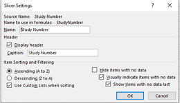
Set sc2 = ActiveWorkbook.SlicerCaches.Add2(tbl, "Study Number")
sc1.Name = "Diluent"
sc2.Name = "StudyNumber"
' Create slicers
Dim sl1 As Slicer
Dim sl2 As Slicer
Set sl1 = sc1.Slicers.Add(ActiveSheet, , "Diluent", "Diluent", 4, 170, 130, 90)
Set sl2 = sc2.Slicers.Add(ActiveSheet, , "Study Number", "Study Number", 4, 310, 140, 134)
End Sub
Button 2
Sub CreateDiluentWorksheetsThenFilter()
Dim ws As Worksheet
Set ws = ActiveSheet
' Define the range of data (including headers)
Dim dataRange As Range
Set dataRange = ws.Range("A11").CurrentRegion
' Sort the data by Diluent column (column H)
dataRange.Sort key1:=Range("H11"), Header:=xlYes
' Find the last row of data
Dim lastRow As Long
lastRow = dataRange.Rows.Count
' Loop through the data and create a new worksheet for each unique Diluent value
Dim diluentDict As Object
Set diluentDict = CreateObject("Scripting.Dictionary")
Dim diluent As String
Dim diluentData As Variant
Dim i As Long
For i = 2 To lastRow
diluent = dataRange.Cells(i, "H").Value
If Not diluentDict.exists(diluent) Then
' Create a new worksheet for this Diluent value
Dim newSheet As Worksheet
Set newSheet = Worksheets.Add(After:=Worksheets(Worksheets.Count))
newSheet.Name = diluent
' Copy the header row to the new worksheet
ws.Range("A11:J11").Copy Destination:=newSheet.Range("A1")
' Add this Diluent value to the dictionary and store the associated data
diluentDict.Add diluent, newSheet
diluentData = dataRange.Rows(i).Value
' Copy the data to the new worksheet
newSheet.Range("A2").Resize(1, UBound(diluentData, 2)).Value = diluentData
' Check if the Diluent value meets the criteria of the "Slicer_Diluent" slicer
If diluent <> slicerValue1 Then
newSheet.Visible = False
End If
Else
' Add this row to the existing Diluent worksheet
diluentData = dataRange.Rows(i).Value
Set newSheet = diluentDict(diluent)
newSheet.Cells(Rows.Count, "A").End(xlUp).Offset(1, 0).Resize(1, UBound(diluentData, 2)).Value = diluentData
End If
Next i
' Get the selected values of the "StudyNumber" slicer
Dim selectedValues As Variant
selectedValues = ActiveWorkbook.SlicerCaches("Slicer_StudyNumber").VisibleSlicerItemsList
' Hide all rows on "Sheet1" that are not selected in the "StudyNumber" slicer
Dim dataRangeShow As Range
Set dataRangeShow = ws.Range("A11").CurrentRegion
dataRangeShow.AutoFilter Field:=6, Criteria1:=Array(selectedValues), Operator:=xlFilterValues
' Clear any existing filters on the new worksheets
Dim sheet As Worksheet
For Each sheet In diluentDict.Items()
sheet.AutoFilterMode = False
Next sheet
End Sub
I am getting a run-time error '5' on the following line:
selectedValues = ActiveWorkbook.SlicerCaches("Slicer_StudyNumber").VisibleSlicerItemsList
I have tried all different versions of the slicer name to no avail.
The first slicer contains the unique values found in column H ("Diluent"). The second slicer contains all unique values found in column J ("Study Number").
The second button will generate new worksheets and copy rows according to the column H value. This works perfectly.
What I would like to happen is that Slicer 2 is used to filter/determine which worksheets and rows are visible to the user. I know an option is just to generate slicer 2 on each worksheet, but I would like to better understand the error that I am getting.
Button 1:
Sub S1ClickToPasteButton_Click()
Dim rng As Range
Dim numRows As Long
Dim colRange As Range
Dim rowCounter As Long
Dim tbl As ListObject
Dim i As Long
Dim j As Long
'Copy data to clipboard
Application.CutCopyMode = False
ActiveSheet.Range("A12").PasteSpecial xlPasteAll
'Set target range for pasting
Set rng = ActiveSheet.Range("A12")
'Get number of rows pasted and adjust target range
numRows = rng.CurrentRegion.Rows.Count
Set rng = rng.Resize(numRows)
'Delete first two columns and shift data left
rng.EntireColumn.Resize(, 2).Delete Shift:=xlShiftToLeft
'Add generic header row
Range("A11").Value = "Compound #"
Range("B11").Value = "Order Number"
Range("C11").Value = "Requestor"
Range("D11").Value = "Date Requested"
Range("E11").Value = "Date Required"
Range("F11").Value = "Requested Lot"
Range("G11").Value = "Amount"
Range("H11").Value = "Diluent"
Range("I11").Value = "Study Number"
Range("J11").Value = "Comments"
'Add table and name it
Set tbl = ActiveSheet.ListObjects.Add(xlSrcRange, Range("A11").CurrentRegion, , xlYes)
tbl.Name = "PastedFromDB" ' Change the name to whatever you want
tbl.TableStyle = "TableStyleMedium2"
tbl.HeaderRowRange.Font.Bold = True
'Resize columns
For i = 1 To tbl.ListColumns.Count
tbl.ListColumns(i).Range.Columns.AutoFit
Next i
'Add dash to blank cells in table
Set colRange = tbl.Range
For j = colRange.Row + 1 To colRange.Row + colRange.Rows.Count - 1
For i = colRange.Column To colRange.Column + colRange.Columns.Count - 1
If IsEmpty(Cells(j, i)) Then
Cells(j, i).Value = "-"
End If
Next i
Next j
'Format column B as numerical
tbl.ListColumns("Order Number").DataBodyRange.NumberFormat = "0"
' Add slicer caches and set names
Dim sc1 As SlicerCache
Dim sc2 As SlicerCache
Set sc1 = ActiveWorkbook.SlicerCaches.Add2(tbl, "Diluent")
Set sc2 = ActiveWorkbook.SlicerCaches.Add2(tbl, "Study Number")
sc1.Name = "Diluent"
sc2.Name = "StudyNumber"
' Create slicers
Dim sl1 As Slicer
Dim sl2 As Slicer
Set sl1 = sc1.Slicers.Add(ActiveSheet, , "Diluent", "Diluent", 4, 170, 130, 90)
Set sl2 = sc2.Slicers.Add(ActiveSheet, , "Study Number", "Study Number", 4, 310, 140, 134)
End Sub
Button 2
Sub CreateDiluentWorksheetsThenFilter()
Dim ws As Worksheet
Set ws = ActiveSheet
' Define the range of data (including headers)
Dim dataRange As Range
Set dataRange = ws.Range("A11").CurrentRegion
' Sort the data by Diluent column (column H)
dataRange.Sort key1:=Range("H11"), Header:=xlYes
' Find the last row of data
Dim lastRow As Long
lastRow = dataRange.Rows.Count
' Loop through the data and create a new worksheet for each unique Diluent value
Dim diluentDict As Object
Set diluentDict = CreateObject("Scripting.Dictionary")
Dim diluent As String
Dim diluentData As Variant
Dim i As Long
For i = 2 To lastRow
diluent = dataRange.Cells(i, "H").Value
If Not diluentDict.exists(diluent) Then
' Create a new worksheet for this Diluent value
Dim newSheet As Worksheet
Set newSheet = Worksheets.Add(After:=Worksheets(Worksheets.Count))
newSheet.Name = diluent
' Copy the header row to the new worksheet
ws.Range("A11:J11").Copy Destination:=newSheet.Range("A1")
' Add this Diluent value to the dictionary and store the associated data
diluentDict.Add diluent, newSheet
diluentData = dataRange.Rows(i).Value
' Copy the data to the new worksheet
newSheet.Range("A2").Resize(1, UBound(diluentData, 2)).Value = diluentData
' Check if the Diluent value meets the criteria of the "Slicer_Diluent" slicer
If diluent <> slicerValue1 Then
newSheet.Visible = False
End If
Else
' Add this row to the existing Diluent worksheet
diluentData = dataRange.Rows(i).Value
Set newSheet = diluentDict(diluent)
newSheet.Cells(Rows.Count, "A").End(xlUp).Offset(1, 0).Resize(1, UBound(diluentData, 2)).Value = diluentData
End If
Next i
' Get the selected values of the "StudyNumber" slicer
Dim selectedValues As Variant
selectedValues = ActiveWorkbook.SlicerCaches("Slicer_StudyNumber").VisibleSlicerItemsList
' Hide all rows on "Sheet1" that are not selected in the "StudyNumber" slicer
Dim dataRangeShow As Range
Set dataRangeShow = ws.Range("A11").CurrentRegion
dataRangeShow.AutoFilter Field:=6, Criteria1:=Array(selectedValues), Operator:=xlFilterValues
' Clear any existing filters on the new worksheets
Dim sheet As Worksheet
For Each sheet In diluentDict.Items()
sheet.AutoFilterMode = False
Next sheet
End Sub
I am getting a run-time error '5' on the following line:
selectedValues = ActiveWorkbook.SlicerCaches("Slicer_StudyNumber").VisibleSlicerItemsList
I have tried all different versions of the slicer name to no avail.
")


