VBA to chose format from one column & speed from different column

dinkss

Board Regular
Joined
Aug 25, 2020
Messages
129
Office Version
  1. 365
  2. 2016
Platform
  1. Windows
Hi there,

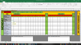
I have excel sheet data created with VBA, and simple dropdown menu list to chose different formats.
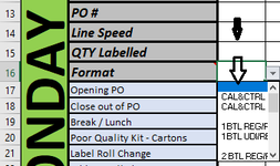
But I would like to have an option to select format and then the line speed for selected format would show on cell on top of it.

Is there any VBA code that I could use or a simple dropdown menu list or macro? Can anyone help?

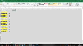
I have attached screenshots of my excel and formats with speeds.

Any help will be much appreciated.
 

Attachments

  • format & line speed all.png
    format & line speed all.png
    205.5 KB · Views: 7
  • format & line speed data.png
    format & line speed data.png
    136.3 KB · Views: 8
  • format & line speed.png
    format & line speed.png
    9.7 KB · Views: 7

Excel Facts

Is there a shortcut key for strikethrough?
Ctrl+S is used for Save. Ctrl+5 is used for Strikethrough. Why Ctrl+5? When you use hashmarks to count |||| is 4, strike through to mean 5.
How about in C14
Excel Formula:
=VLOOKUP(C16,DATA_PULL!$A$3:$B$50,2,0)
 
Upvote 0
How about in C14
Excel Formula:
=VLOOKUP(C16,DATA_PULL!$A$3:$B$50,2,0)
Works great buddy.

Can you explain to me why you have entered this: $B$50,2,0 in the code? I presume it is only the range from A3 to B50 yes?
 
Upvote 0
That's right, in your image the range only goes down to row 25 so I added a few more rows for safety.
 
Upvote 0
How about in C14
Excel Formula:
=VLOOKUP(C16,DATA_PULL!$A$3:$B$50,2,0)


Your formula [=VLOOKUP(C16,DATA_PULL!$A$3:$B$50,2,0)] works fine but now I’m getting error with calculating data in cells:
Q10 = =SUM(C10:P10)
Q12 = =SUM(C12:P12)
Q14 = =IFERROR(AVERAGE(C14:P14),"")

How can I avoid getting errors and change formula to calculate SUM from C10:P10 in Q10 ?
How can I avoid getting errors and change formula to calculate SUM from C12:P12 in Q12 ?
How can I avoid getting errors and change formula to calculate AVERAGE from C14:P14 in Q14 ?

Before using VLOOKUP everything was fine but now, with vlookup option formulas are not working anymore :(
 

Attachments

  • formulas-errors.png
    formulas-errors.png
    188.3 KB · Views: 9
Upvote 0
How about
Excel Formula:
=IF(C16="","",VLOOKUP(C16,DATA_PULL!$A$3:$B$50,2,0))
 
Upvote 0
How about
Excel Formula:
=IF(C16="","",VLOOKUP(C16,DATA_PULL!$A$3:$B$50,2,0))
Now it works fine for Q14 cell, but it still gives errors for:
Q10 = =SUM(C10:P10)
Q12 = =SUM(C12:P12)
 
Upvote 0
What formula do you have in those rows?
 
Upvote 0
I meant the formula that is return the #N/A
 
Upvote 0

Forum statistics

Threads
1,214,954
Messages
6,122,461
Members
449,085
Latest member
ExcelError

We've detected that you are using an adblocker.

We have a great community of people providing Excel help here, but the hosting costs are enormous. You can help keep this site running by allowing ads on MrExcel.com.
Allow Ads at MrExcel

Which adblocker are you using?

Disable AdBlock

Follow these easy steps to disable AdBlock

1)Click on the icon in the browser’s toolbar.
2)Click on the icon in the browser’s toolbar.
2)Click on the "Pause on this site" option.
Go back

Disable AdBlock Plus

Follow these easy steps to disable AdBlock Plus

1)Click on the icon in the browser’s toolbar.
2)Click on the toggle to disable it for "mrexcel.com".
Go back

Disable uBlock Origin

Follow these easy steps to disable uBlock Origin

1)Click on the icon in the browser’s toolbar.
2)Click on the "Power" button.
3)Click on the "Refresh" button.
Go back

Disable uBlock

Follow these easy steps to disable uBlock

1)Click on the icon in the browser’s toolbar.
2)Click on the "Power" button.
3)Click on the "Refresh" button.
Go back
Back
Top