VBA to copy rows from 5 sheets and paste on a separate sheet at a specific starting range

TomK58

New Member
Joined
May 18, 2020
Messages
9
Office Version
  1. 365
Platform
  1. Windows
I'd like to copy multiple rows on five separate worksheets and copy them onto a 6th worksheet at a specific starting cell range. The code i'm working with now is below. It currently copies multiple rows and columns from one sheet based on the variables requested, from s1 to a blank s2. I really need it to paste to a different sheet at a specific starting range. I would also like to add the exact same variable request to s3, s4, s5, s6, then paste the results of all 5 on to a 7th sheet labeled "Proposal" but paste them beginning at a specific cell range of A310 then fill downward from there. The reason I'm pasting them at a specific starting range is because I have other data on the same "Proposal" sheet that I don't want to interfere with or overwrite. The variable for the copy selection is (copy columns C,D & E in any rows with a value of more than 0 in column E). Below is the current macro that copies from sheet 1 and pastes to a blank sheet s2:
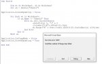

Sub TomK58()


Dim s1 As Worksheet, s2 As Worksheet
Set s1 = Sheets("Commercial Video")
Set s2 = Sheets("Sheet2")
Dim i As Long, lr As Long
Dim lr2 As Long
lr = s1.Range("E" & Rows.Count).End(xlUp).Row
Application.ScreenUpdating = False
For i = 1 To lr
If s1.Range("E" & i) > 0 Then
s1.Range("C" & i & ":E" & i).Copy
lr2 = s2.Range("A" & Rows.Count).End(xlUp).Row
s2.Range("A" & lr2 + 1).PasteSpecial xlPasteValues
End If
Next i
Application.CutCopyMode = False
Application.ScreenUpdating = True
MsgBox "Action Completed"

End Sub

I'm on a VBA learning fast track, but have a long way to go. Thanks if advance for any help!

Thank you advance for your help and guidance!
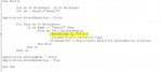
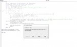
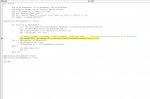
 

Excel Facts

Format cells as currency
Select range and press Ctrl+Shift+4 to format cells as currency. (Shift 4 is the $ sign).
Hello Tom,

Try the following code:-

VBA Code:
Sub Test()

        Dim ws As Worksheet, sh As Worksheet
        Set sh = Sheets("Proposal")
        
Application.ScreenUpdating = False
        
        For Each ws In Worksheets
              If ws.Name <> "Proposal" Then
                    With ws.[A1].CurrentRegion
                           .AutoFilter 5, ">" & 0
                           .Columns("C:E").Offset(1).Copy
                           sh.Range("A" & Rows.Count).End(3)(2).PasteSpecial xlValues
                    End With
              End If
        Next ws
        
Application.CutCopyMode = False
Application.ScreenUpdating = True

End Sub

I'm assuming:-
- The data in all the source sheets begins in Row2 with headings in Row1.
- The data currently in the destination sheet (Proposal) finishes in Row309.

If my assumptions are incorrect, then please let me know.

Test the code in a copy of your workbook first.

I hope that this helps.

Cheerio,
vcoolio.
 
Upvote 0
vcoolio, Thanks for your help! Your assumptions are correct. However I failed to mention that I have other worksheets in the same workbook. I'm testing with a copy and added Sheet2 then edited the two instances of "proposal" to "Sheet2" as a first run to see if the code would copy to A310. I receive a runtime 1004 error that fails on AutoFiliter (see attached). Also wanted to clarify that the variable I'll need to have is to copy only rows with a value of more than 0 in column E.

I appreciate your help!

TomK58
 

Attachments

  • Screen Shot 2020-05-28 at 12.04.07 AM.jpg
    Screen Shot 2020-05-28 at 12.04.07 AM.jpg
    50.4 KB · Views: 2
  • Screen Shot 2020-05-28 at 12.04.17 AM.jpg
    Screen Shot 2020-05-28 at 12.04.17 AM.jpg
    41 KB · Views: 2
Upvote 0
Hello Tom,

I've tested the code in a mock-up of what I assume your workbook to look like and the code does exactly what it should. However, your workbook may have a totally different set out.
It would be worthwhile if you uploaded a sample copy of your actual workbook showing inputs and outputs. A few lines per source sheet will suffice.
Upload your sample to a file sharing site such as Drop Box or WeTransfer then post the link to your file back here. If your data is sensitive then please use dummy data. Make sure that the sample is an exact replica of your actual workbook.

Rich (BB code):
"However I failed to mention that I have other worksheets in the same workbook."
Exactly what are all the source sheets named? Is there only one destination sheet ("Proposal")? Are there other worksheets in the workbook that need to be excluded from the process?

Rich (BB code):
"............................is to copy only rows with a value of more than 0 in column E."
That's exactly what the code does.

BTW, I've missed out one line in the code above. Add this:-

VBA Code:
.AutoFilter

directly after this line:-

VBA Code:
sh.Range("A" & Rows.Count).End(3)(2).PasteSpecial xlValues

The extra line turns off the autofilter.

Cheerio,
vcoolio.
 
Upvote 0
vcoolio,

Thanks! I tried adding the extra line but it still hangs at the same spot. Below is a link to the file so you can take a look at it. The source sheets are "Residential", "Commercial_Intrusion", "Commercial_Fire", "Commercial_Video" and "Commercial_Access_Control". The destination sheet is "Commercial_Quote" beginning at A310
Thanks again for you help!

TomK58
 
Upvote 0
Hello Tom,

Your workbook is considerably different from what I imagined. It is heavily loaded with formatting, merged cells etc. which in turn has made your workbook rather bloated and difficult to work with in terms of VBA.
However, the following code will work:-

VBA Code:
Sub Test()

        Dim ws As Worksheet, sh As Worksheet, sht As Worksheet
        Dim shRng As Range, cAr As Variant, pAr As Variant
        Dim lr As Long, nr As Long, i As Long
        Set ws = Sheets("Sheet List")
        Set sh = Sheets("Commercial_Quote")
        Set shRng = ws.Range("ShList")
       
Application.ScreenUpdating = False
       
        For Each sht In Worksheets
                lr = sht.Cells.Find("*", searchorder:=xlByRows, searchdirection:=xlPrevious).Row
                nr = sh.Cells(Rows.Count, 1).End(xlUp).Row + 1
                cAr = Array("C3:C" & lr, "D3:D" & lr, "E3:E" & lr)
                pAr = Array("B", "C", "A")
              
                If shRng.Find(What:=sht.Name, LookAt:=xlWhole) Is Nothing Then '---->Excludes unwanted worksheets from the search.
                sht.Range("E2", sht.Range("E" & sht.Rows.Count).End(xlUp)).AutoFilter 1, ">0"
        For i = LBound(cAr) To UBound(cAr)
                sht.Range(cAr(i)).Copy
                sh.Range(pAr(i) & nr).PasteSpecial xlValues
        Next i
                sht.[E2].AutoFilter
                End If
        Next sht
       
Application.CutCopyMode = False
Application.ScreenUpdating = True

End Sub

but there are a few things you must do to ensure it works correctly:-
- All cells from row309 down in the "Commercial_Quote" sheet must be un-merged. Merged cells create havoc with vba codes. These cells can be adequately formatted without merging.
- Create a new sheet and name it "Sheet List" (see the 'ws' variable above). I used your former Sheet2 in this case while testing as it is not needed.
- In cell A1 of the "Sheet List" worksheet, place the heading ShList (see the variable 'ShRng' above). From A2 down, place the names of the sheets that need to be excluded from this process; i.e.
"Commercial_Quote", "Scope", "Lists", "Tech Pg", "Start_Quote", "Sheet List", "Engine".
- Select the list of sheet names and go to the Fomulas tab and select "Define Name" from the Defined Names group. A dialogue box will appear. In the name box, "ShList" should appear as should the selected range in the "Refers To" box. Click OK.
- With the list still selected, go to the Insert tab and select Table. The range of the list should appear in the "Where is the data for your table?" box. Ensure that the "My table has headers" box is ticked. You now have a table to which you can add or remove sheets from as the need arises with no need to alter/modify the code in future. Click OK.

Also, some of the source sheets have a number value in Column E but do not have the adjacent details in Columns A:D. Remove these values until they are required as they will give you partial blank rows in the Commercial_Quote sheet.

I hope that this helps.

Cheerio,
vcoolio.
 
Upvote 0
vcoolio,

A huge thank you for your help on this! everything runs great except for an error I receive when the code attempts to paste to the "Commercial_Quote" worksheet. I receive a Run-Time error 1004 (see attached) and the data does not paste to the "Commercial_Quote" worksheet. When I select Debug it refers to the sh.Range paste line. I tried a test by changing the sh from Commercial_Quote to a blank worksheet labeled "Sheet2". When I ran the macro like that, I still received the error but it pasted the expected data to "Sheet2" beginning at row A2. If I enter text or values anywhere on Sheet2 and run again, I receive the same error, but the data does paste beginning at one row below where I entered text. Is there any way to paste the the copied data beginning at A310 regardless of any other condition? FYI - I expect to have additional text pre-formatted further down the sheet on rows that I don't expect the copied data to reach.

Again, I really appreciate you assistance
 

Attachments

  • Screen Shot 2020-05-29 at 7.29.52 AM.jpg
    Screen Shot 2020-05-29 at 7.29.52 AM.jpg
    115.9 KB · Views: 5
  • Screen Shot 2020-05-29 at 7.30.02 AM.jpg
    Screen Shot 2020-05-29 at 7.30.02 AM.jpg
    111.3 KB · Views: 6
Upvote 0
Hello Tom,

The yellow high-lighted line does not refer to the paste line of code. I believe that your version of Excel is 2003 and that message refers to the fact that you have merged cells.

So I'm assuming that the merged cells are causing the problem. Refer to my post #6 again.

I've attached your file here with the code implemented and the changes made as per my post #6. You'll see that the code works as it should.
I've placed a button on the Commercial_Quote sheet. Click on it to see it all work.

Cheerio,
vcoolio.
 
Upvote 0
vcoolio,

That makes sense! I'm actually running Office 365. I didn't realize that some VBA runs a bit differently depending on the Excel version. I'll work on the formatting to eliminate the merged cells. Thanks for taking the time to mock up a button and sending me the file.

Thanks for all your help! Hoping that in time I can develop skills to pass on help to others!

Tom
 
Upvote 0
No worries Tom. You're welcome.

It may be worth upgrading Excel to the latest version.

Personally, I would go through the entire workbook and remove as much formatting as possible, especially merged cells. I know it looks attractive but practicality needs to take precedence.

It may be worth, when you have some spare time, to "google" something like "problems with excessive formatting excel". It's generally good reading (depending on how geeky one might be) and various experts give their biased/unbiased opinions on the subject of formatting. During lock-down it may be a way of idling the time away!

Good luck Tom

Cheerio,
vcoolio.

P.S. : BTW Tom, with each transfer of data to the Commercial_Quote sheet, you may want to clear the previous data. If you need help with that, let us know. We can include another line of code to do that.
 
Last edited:
Upvote 0

Forum statistics

Threads
1,214,653
Messages
6,120,751
Members
448,989
Latest member
mariah3

We've detected that you are using an adblocker.

We have a great community of people providing Excel help here, but the hosting costs are enormous. You can help keep this site running by allowing ads on MrExcel.com.
Allow Ads at MrExcel

Which adblocker are you using?

Disable AdBlock

Follow these easy steps to disable AdBlock

1)Click on the icon in the browser’s toolbar.
2)Click on the icon in the browser’s toolbar.
2)Click on the "Pause on this site" option.
Go back

Disable AdBlock Plus

Follow these easy steps to disable AdBlock Plus

1)Click on the icon in the browser’s toolbar.
2)Click on the toggle to disable it for "mrexcel.com".
Go back

Disable uBlock Origin

Follow these easy steps to disable uBlock Origin

1)Click on the icon in the browser’s toolbar.
2)Click on the "Power" button.
3)Click on the "Refresh" button.
Go back

Disable uBlock

Follow these easy steps to disable uBlock

1)Click on the icon in the browser’s toolbar.
2)Click on the "Power" button.
3)Click on the "Refresh" button.
Go back
Back
Top