VBA to Delete rows if missing values across multiple columns

ENicklin

New Member
Joined
Oct 2, 2021
Messages
11
Office Version
  1. 2019
Platform
  1. Windows
Hello,

I need to search through data from an online database and filter it based on certain criteria than can appear in multiple columns. I have copied the data into an excel sheet and the first batch is about 4k rows long and I probably only need to keep about 25% of that. My sheet is currently 7 columns wide (A-G) I need a code to search columns C, D, E and G and only keep the rows that have the following terms in them:

Cornerstone on Booth
A Different Street (JHS program)
Centre 507
Centretown CHC
Carleton University
ODSP
Emergency Medical Services
Friendship Centre, ODAWA
Haven Youth
JF Norwood, Eliz Fry
Library , Ottawa
ODAWA Native Friendship Centre
ODSP
Ontario Works
Ottawa Police
Somerset West CHC
St.Lukes
SWCHC
Tom Brown Arena
Well , The
YMCA
YMCA Employment Centre
Other (Please Specify)

I need to keep all the rows that have any of these terms in columns C, D, E, and G but if the terms are missing in all the columns then I want to delete the rows. I have found solutions to delete rows based on searches but not to keep rows and delete everything else and when I tried editing the code I just ended up deleting everything.

Any help is appreciated. Cheers,
 

Excel Facts

Difference between two dates
Secret function! Use =DATEDIF(A2,B2,"Y")&" years"&=DATEDIF(A2,B2,"YM")&" months"&=DATEDIF(A2,B2,"MD")&" days"
Hi ENicklin,

Try this (initially on a copy of your data as the results cannot be undone if they're not as expected) where each of the 23 text items are in Col. A of the 'wsLookup' tab:

VBA Code:
Option Explicit
Sub Macro1()

    Dim wsData As Worksheet, wsLookup As Worksheet
    Dim lngMyRow As Long, lngLastRow As Long
    Dim dblResult As Double
    Dim varMyCol As Variant
    
    Application.ScreenUpdating = False
    
    Set wsData = ThisWorkbook.Sheets("Sheet1") 'Sheet name that has the data in columns C, D, E and G. Change to suit if necessary.
    Set wsLookup = ThisWorkbook.Sheets("Sheet2") 'Sheet name that has filter criteria. Change to suit if necessary.
    
    If WorksheetFunction.CountA(wsData.Cells) = 0 Then
        MsgBox "There is no data in """ & wsData.Name & """ to work with.", vbExclamation
        Exit Sub
    End If
    
    lngLastRow = wsData.Cells.Find("*", SearchOrder:=xlByRows, SearchDirection:=xlPrevious).Row
    For lngMyRow = lngLastRow To 2 Step -1 'Assumes the fist row of data is 2 (1 being for headers). Change to suit if necessary.
        For Each varMyCol In Array("C", "D", "E", "G") 'Columns with possible filter criteria. Change to suit if necessary.
            dblResult = dblResult + Application.WorksheetFunction.CountIf(wsLookup.Range("A:A"), wsData.Range(CStr(varMyCol) & lngMyRow)) 'Assumes criteria are in column A of 'wsLookup'. Change to suit if necessary.
            If dblResult > 0 Then
                Exit For
            End If
        Next varMyCol
        If dblResult = 0 Then
            wsData.Rows(lngMyRow).Delete
        End If
        dblResult = 0
    Next lngMyRow
    
    Application.ScreenUpdating = True

End Sub

Regards,

Robert
 
Upvote 0
Solution
It would be good to have a sample of say 10-15 rows of sample data. For one thing, that would probably clarify whether the cells contain exactly the things in your list or could include, say, "Ottawa Police Department" and if so whether that row should get kept or deleted. It would also save helpers o lot of time manually typing data to test with. ;)

MrExcel has a tool called “XL2BB” that lets you post samples of your data that will allow us to copy/paste it to our Excel spreadsheets, so we can work with the same copy of data that you are. Instructions on using this tool can be found here: XL2BB Add-in

Note that there is also a "Test Here” forum on this board. This is a place where you can test using this tool (or any other posting techniques that you want to test) before trying to use those tools in your actual posts.

Also, is the list in post 1 recorded in the workbook somewhere?
 
Upvote 0
I made a dynamic version of this using the Advanced Filter (which I learned about today) in VBA. The video below shows how to use and how dynamic this is! (So I guess this is a second option.)

VBA Code:
Sub Delete_Rows()

'Input
'Dim tableRangeAddress_IncludingHeaderRow As String '$A$2:$G$8
'tableRangeAddress_IncludingHeaderRow = "A2:G8"

Dim tableRangeAddress_IncludingHeaderRow As String
tableRangeAddress_IncludingHeaderRow = RangeSelectionPrompt("Select the entire table range (including header row)")

If tableRangeAddress_IncludingHeaderRow = "" Then Exit Sub

Dim header_Field_RowNumber As Long
header_Field_RowNumber = Range(tableRangeAddress_IncludingHeaderRow)(1, 1).Row

Dim firstDataRow As Long
firstDataRow = header_Field_RowNumber + 1

Dim lastColumnNumber As Integer 'Last column number in original table.
lastColumnNumber = Range(tableRangeAddress_IncludingHeaderRow)(1, Range(tableRangeAddress_IncludingHeaderRow).Columns.Count).Column

Dim lastDataRow As Long 'Last row number in original table.
lastDataRow = Range(tableRangeAddress_IncludingHeaderRow)(Range(tableRangeAddress_IncludingHeaderRow).Rows.Count, 1).Row

'=SUM(IF(TRANSPOSE(ISNA(MATCH($I$2:$I$4,INDEX(FILTER(IF($A$1:$G$1=1,$A$3:$G$8,""),
'INDEX(IF($A$1:$G$1=1,$A$3:$G$8,""),MATCH(J3,$J$3:J$8,0),0)<>""),MATCH(J3,$J$3:J$8,0),0),0)))=FALSE,1,0))

Dim tableRangeAddress_ExcludingHeaderRow As String '$A$3:$G$8
tableRangeAddress_ExcludingHeaderRow = _
Range(tableRangeAddress_IncludingHeaderRow)(2, 1).Address & ":" & _
Range(tableRangeAddress_IncludingHeaderRow)(Range(tableRangeAddress_IncludingHeaderRow).Rows.Count, _
                                            Range(tableRangeAddress_IncludingHeaderRow).Columns.Count _
                                            ).Address
Dim rowAddressWithThe_1s As String '$A$1:$G$1
rowAddressWithThe_1s = Range(tableRangeAddress_IncludingHeaderRow).Rows(1).Offset(-1, 0).Address

'Place a criteria column one column over from the last column in the original data.
    'For now, just identify the column letter and place the Criteria field name, which we can just call "Criteria".
    Dim columnLetter_ToPutCriteriaColumnFormula As String
    columnLetter_ToPutCriteriaColumnFormula = Split(Cells(1, lastColumnNumber + 1).Address, "$")(1)
    Range(columnLetter_ToPutCriteriaColumnFormula & header_Field_RowNumber).Value = "Criteria"

'Column with keywords.
Dim columnLetter_To_Retrieve_KeywordsFrom As String
columnLetter_To_Retrieve_KeywordsFrom = Split(Cells(1, lastColumnNumber + 2).Address, "$")(1)

Dim firstRowWithAKeyWord As Long '2
firstRowWithAKeyWord = Cells(1, columnLetter_To_Retrieve_KeywordsFrom).End(xlDown).Row

Dim lastRowWithAKeyWord As Long '4
lastRowWithAKeyWord = Cells(ActiveSheet.Rows.Count, columnLetter_To_Retrieve_KeywordsFrom).End(xlUp).Row

'Column letter to place the criteria field name and criteria conditional
Dim columnLetter_Of_Criteria_Range As String
columnLetter_Of_Criteria_Range = Split(Cells(1, lastColumnNumber + 3).Address, "$")(1)

'Place criteria cell (and its header).
Range(columnLetter_Of_Criteria_Range & header_Field_RowNumber - 1).Value = "Criteria"
Range(columnLetter_Of_Criteria_Range & header_Field_RowNumber).Formula = "=" & Chr(34) & ">0" & Chr(34)

    'Define this address for the Advanced Filter (for later)
    Dim criteriaRangeAddress As String
    criteriaRangeAddress = columnLetter_Of_Criteria_Range & header_Field_RowNumber - 1 & ":" & columnLetter_Of_Criteria_Range & header_Field_RowNumber

'Column letter to place row counter.  For compactness, just put in the same column as the criteria range.
Dim columnLetter_ToPutRowCounterFormula As String
columnLetter_ToPutRowCounterFormula = columnLetter_Of_Criteria_Range

'Fill the criteria column.
With Range(columnLetter_ToPutCriteriaColumnFormula & firstDataRow & ":" & columnLetter_ToPutCriteriaColumnFormula & lastDataRow)
    .Formula = "=SUM(IF(TRANSPOSE(ISNA(MATCH(" & "$" & columnLetter_To_Retrieve_KeywordsFrom & "$" & firstRowWithAKeyWord & ":" & "$" & columnLetter_To_Retrieve_KeywordsFrom & "$" & lastRowWithAKeyWord & ",INDEX(FILTER(IF(" & rowAddressWithThe_1s & "=1," & tableRangeAddress_ExcludingHeaderRow & "," & Chr(34) & Chr(34) & "),INDEX(IF(" & rowAddressWithThe_1s & "=1," & tableRangeAddress_ExcludingHeaderRow & "," & Chr(34) & Chr(34) & "),MATCH(" & columnLetter_ToPutRowCounterFormula & firstDataRow & "," & "$" & columnLetter_ToPutRowCounterFormula & "$" & firstDataRow & ":" & columnLetter_ToPutRowCounterFormula & "$" & lastDataRow & ",0),0)<>" & Chr(34) & Chr(34) & "),MATCH(" & columnLetter_ToPutRowCounterFormula & firstDataRow & "," & "$" & columnLetter_ToPutRowCounterFormula & "$" & firstDataRow & ":" & columnLetter_ToPutRowCounterFormula & "$" & lastDataRow & ",0),0),0)))=FALSE,1,0))"
    .Replace What:="@", Replacement:="", LookAt:=xlPart, FormulaVersion:=xlReplaceFormula2
End With

'Fill the row counter column.
Range(columnLetter_ToPutRowCounterFormula & firstDataRow & ":" & columnLetter_ToPutRowCounterFormula & lastDataRow).Formula = "=ROW()"


'Append a column letter to the original table range address.
Dim firstColumnLetter_Of_OriginalTableAddress As String
firstColumnLetter_Of_OriginalTableAddress = Split(Range(tableRangeAddress_IncludingHeaderRow)(1, 1).Address, "$")(1)

tableRangeAddress_IncludingHeaderRow = firstColumnLetter_Of_OriginalTableAddress & header_Field_RowNumber & ":" & columnLetter_ToPutCriteriaColumnFormula & lastDataRow

'Copy to range
Dim topLeft_CellAddress_ToPaste As String 'Make it paste in the same start row, 5 columns to the right.
topLeft_CellAddress_ToPaste = Range(Split(Cells(header_Field_RowNumber, lastColumnNumber + 5).Address, "$")(1) & header_Field_RowNumber).Address

Dim columnLetterOfPastedResult_Where_Criteria_Column_Is As String
columnLetterOfPastedResult_Where_Criteria_Column_Is = Split(Cells(header_Field_RowNumber, lastColumnNumber + Range(topLeft_CellAddress_ToPaste).Column).Address, "$")(1)

'Clear the contents in that rectangular portion of the sheet ONLY.
Range(topLeft_CellAddress_ToPaste & ":" & columnLetterOfPastedResult_Where_Criteria_Column_Is & lastDataRow).ClearContents

'Advanced filter
Range(tableRangeAddress_IncludingHeaderRow).AdvancedFilter _
Action:=xlFilterCopy, _
CriteriaRange:=Range(criteriaRangeAddress), _
CopyToRange:=Range(topLeft_CellAddress_ToPaste), _
Unique:=False

'Delete all helper column values/formulas.
Range(columnLetter_ToPutCriteriaColumnFormula & firstDataRow - 1 & ":" & columnLetter_ToPutCriteriaColumnFormula & lastDataRow).ClearContents
Range(columnLetter_ToPutRowCounterFormula & firstDataRow - 2 & ":" & columnLetter_ToPutRowCounterFormula & lastDataRow).ClearContents
Range(columnLetterOfPastedResult_Where_Criteria_Column_Is & firstDataRow - 1 & ":" & columnLetterOfPastedResult_Where_Criteria_Column_Is & lastDataRow).ClearContents

End Sub

Sub Test__RangeSelectionPrompt()
MsgBox RangeSelectionPrompt("Choose Cells")
End Sub
Function RangeSelectionPrompt(titleOfRangeSelectionPromptBox As String)
'Code is from http://www.vbaexpress.com/forum/showthread.php?763-Solved-Inputbox-Cell-Range-selection-Nothing-selected-or-Cancel&p=6680&viewfull=1#post6680

Dim Selectedarea As Range
On Error Resume Next
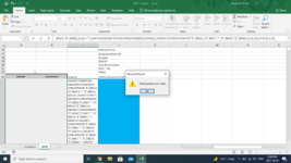
Set Selectedarea = Application.InputBox(prompt:="Left click on the top-left cell and drag to the botSomething-right cell.", _
Title:=titleOfRangeSelectionPromptBox, Default:=Selection.Address, Type:=8)

'If the user clicked on cancel,
If Selectedarea Is Nothing Then
    Selectedarea = ""
    Exit Function
End If

RangeSelectionPrompt = Selectedarea.Address

End Function
 
Upvote 0
It would be good to have a sample of say 10-15 rows of sample data. For one thing, that would probably clarify whether the cells contain exactly the things in your list or could include, say, "Ottawa Police Department" and if so whether that row should get kept or deleted. It would also save helpers o lot of time manually typing data to test with. ;)

MrExcel has a tool called “XL2BB” that lets you post samples of your data that will allow us to copy/paste it to our Excel spreadsheets, so we can work with the same copy of data that you are. Instructions on using this tool can be found here: XL2BB Add-in

Note that there is also a "Test Here” forum on this board. This is a place where you can test using this tool (or any other posting techniques that you want to test) before trying to use those tools in your actual posts.

Also, is the list in post 1 recorded in the workbook somewhere?
The list wasn't previosly recorded but I have since added a tab with that list. I have attached a screenshot with the names and dates removed. I can't upload a minisheet because I am on a work computer and cannot install any software. Hopefully that helps. Also the names for the locations I included in post 1 are exactly how they are written in the document. Thanks.

1633479221766.png
 
Upvote 0
Also, here's how to do this without VBA (in Office 365, which I see you have). Set up the formulas in a sheet in the following way.

See this video for an explanation on how it works and how to use the Advanced Filter in the Data Ribbon.

But what I did not mention in the video (which you need to know) is:
  • Only input parameters into cells B1, B2, B3, B4, and "mark the 1s". In the video, they are in row 17 and can stay there if you don't move the header row of the table up or down.
    • All other numbers in Column B are parameters calculated from what you input in cells B1:B4 and used by the BIG formulas.
  • You need to fill down the formulas that are in K19 and I19 to the bottom of your data.

Blank - Copy.xlsb
ABCDEFGHIJK
1Top Left Corner of TableB18Keywords:
2Bottom Right Corner of TableI23A
3Top Keyword CellJ2B
4Bottom Keyword CellJ4C
5Row with the 1's17
6Column Heading Row18
7First Data Row19
8Last Data Row23
9First Column LetterB
10Last Column LetterH
11Criteria Column column letterI
12Keyword column letterJ
13First keyword Row2
14Last keyword Row4
15Criteria Range column LetterK
16
171111Criteria
18f1f2f3f4f5f6f7Criteria>0
19XXXXAXX119
20AXXXXXX020
21BBXXCXX121
22CBCXXXX122
23DXXXXXX023
Sheet3 (10)
Cell Formulas
RangeFormula
B5B5=ROW(INDIRECT(B1))-1
B6:B7B6=B5+1
B8B8=ROW(INDIRECT($B$2))
B9B9=SUBSTITUTE(SUBSTITUTE(ADDRESS(1,COLUMN(OFFSET(INDIRECT(CONCATENATE($B$1,"1")),0,0))),"$",""),"1","")
B10B10=SUBSTITUTE(SUBSTITUTE(ADDRESS(1,COLUMN(OFFSET(INDIRECT(CONCATENATE($B$2,"1")),0,-1))),"$",""),"1","")
B11B11=SUBSTITUTE(SUBSTITUTE(ADDRESS(1,COLUMN(OFFSET(INDIRECT(CONCATENATE($B$10,"1")),0,1))),"$",""),"1","")
B12B12=SUBSTITUTE(SUBSTITUTE(ADDRESS(1,COLUMN(OFFSET(INDIRECT(CONCATENATE($B$10,"1")),0,2))),"$",""),"1","")
B13B13=ROW(INDIRECT($B$3))
B14B14=ROW(INDIRECT($B$4))
B15B15=SUBSTITUTE(SUBSTITUTE(ADDRESS(1,COLUMN(OFFSET(INDIRECT(CONCATENATE($B$10,"1")),0,3))),"$",""),"1","")
I19:I23I19=SUM(IF(TRANSPOSE(ISNA(MATCH(INDIRECT(CONCATENATE("$",$B$12,"$",$B$13,":","$",$B$12,$B$14)),INDEX(FILTER(IF(INDIRECT(CONCATENATE("$",$B$9,"$",$B$5,":","$",$B$10,"$",$B$5))=1,INDIRECT(CONCATENATE("$",$B$9,"$",$B$7,":","$",$B$10,"$",$B$8)),""),INDEX(IF(INDIRECT(CONCATENATE("$",$B$9,"$",$B$5,":","$",$B$10,"$",$B$5))=1,INDIRECT(CONCATENATE("$",$B$9,"$",$B$7,":","$",$B$10,"$",$B$8)),""),MATCH(INDIRECT(CONCATENATE($B$15,ROW())),INDIRECT(CONCATENATE("$",$B$15,"$",$B$7,":","$",$B$15,"$",$B$8)),0),0)<>""),MATCH(INDIRECT(CONCATENATE($B$15,ROW())),INDIRECT(CONCATENATE("$",$B$15,"$",$B$7,":","$",$B$15,"$",$B$8)),0),0),0)))=FALSE,1,0))
K18K18=">0"
K19:K23K19=ROW()
 
Upvote 0
Thanks for the reply. So I tried this out and I get an error with the formula for the criteria column. Spcifically it highlights the first filter term and says that is not a valid function.

1633484341385.png
 

Attachments

  • 1633484318938.png
    1633484318938.png
    153.4 KB · Views: 10
Upvote 0
It looks like you didn't put the formulas in the top left. (In my sheet A1:B15.) Please put those in first and then put the BIG formula in, as the BIG formula depends on those.

Edit:

And before you put those smaller formulas in (B5:B15) in, you have just put some values in B1:B4 like I have first. Then change them afterwards! (Sorry for the confusion!)

Also, it's kind of confusing, but you have to input the tiny formula that's in B6 in and then fill down to B7.
 
Last edited:
Upvote 0
Please see my edits to my last post. But in addition, you also need to type in the word Criteria in both cells that it appears. (The Advanced Filter won't work as shown in the video otherwise.) If you want to call it something else besides "Criteria", that's okay. Just make sure that both cells have the same thing typed in them (non-blank).

So your sheet should look something like this after you're ready to copy the data in.

(And if you want to move the cells B1:B15 somewhere else, you can, but CUT and paste them whereever you want to move them so that all formulas remain linked.)

Blank - Copy.xlsb
ABCDEFGHIJK
1B18Cornerstone on Booth
2I23A Different Street (JHS program)
3J1Centre 507
4J23Centretown CHC
517Carleton University
618ODSP
719Emergency Medical Services
823Friendship Centre, ODAWA
9BHaven Youth
10HJF Norwood, Eliz Fry
11ILibrary , Ottawa
12JODAWA Native Friendship Centre
131ODSP
1423Ontario Works
15KOttawa Police
16Somerset West CHC
171111St.LukesCriteria
18DateClientFromToReferrerDeniedCommentsCriteriaSWCHC>0
190Tom Brown Arena19
200Well , The20
210YMCA21
220YMCA Employment Centre22
230Other (Please Specify)23
24024
25025
26026
27027
28028
29029
30030
31031
32032
Sheet14
Cell Formulas
RangeFormula
B5B5=ROW(INDIRECT(B1))-1
B6:B7B6=B5+1
B8B8=ROW(INDIRECT($B$2))
B9B9=SUBSTITUTE(SUBSTITUTE(ADDRESS(1,COLUMN(OFFSET(INDIRECT(CONCATENATE($B$1,"1")),0,0))),"$",""),"1","")
B10B10=SUBSTITUTE(SUBSTITUTE(ADDRESS(1,COLUMN(OFFSET(INDIRECT(CONCATENATE($B$2,"1")),0,-1))),"$",""),"1","")
B11B11=SUBSTITUTE(SUBSTITUTE(ADDRESS(1,COLUMN(OFFSET(INDIRECT(CONCATENATE($B$10,"1")),0,1))),"$",""),"1","")
B12B12=SUBSTITUTE(SUBSTITUTE(ADDRESS(1,COLUMN(OFFSET(INDIRECT(CONCATENATE($B$10,"1")),0,2))),"$",""),"1","")
B13B13=ROW(INDIRECT($B$3))
B14B14=ROW(INDIRECT($B$4))
B15B15=SUBSTITUTE(SUBSTITUTE(ADDRESS(1,COLUMN(OFFSET(INDIRECT(CONCATENATE($B$10,"1")),0,3))),"$",""),"1","")
I19:I32I19=SUM(IF(TRANSPOSE(ISNA(MATCH(INDIRECT(CONCATENATE("$",$B$12,"$",$B$13,":","$",$B$12,$B$14)),INDEX(FILTER(IF(INDIRECT(CONCATENATE("$",$B$9,"$",$B$5,":","$",$B$10,"$",$B$5))=1,INDIRECT(CONCATENATE("$",$B$9,"$",$B$7,":","$",$B$10,"$",$B$8)),""),INDEX(IF(INDIRECT(CONCATENATE("$",$B$9,"$",$B$5,":","$",$B$10,"$",$B$5))=1,INDIRECT(CONCATENATE("$",$B$9,"$",$B$7,":","$",$B$10,"$",$B$8)),""),MATCH(INDIRECT(CONCATENATE($B$15,ROW())),INDIRECT(CONCATENATE("$",$B$15,"$",$B$7,":","$",$B$15,"$",$B$8)),0),0)<>""),MATCH(INDIRECT(CONCATENATE($B$15,ROW())),INDIRECT(CONCATENATE("$",$B$15,"$",$B$7,":","$",$B$15,"$",$B$8)),0),0),0)))=FALSE,1,0))
K18K18=">0"
K19:K32K19=ROW()
 
Last edited:
Upvote 0
Please see my edits to my last post. But in addition, you also need to type in the word Criteria in both cells that it appears. (The Advanced Filter won't work as shown in the video otherwise.) If you want to call it something else besides "Criteria", that's okay. Just make sure that both cells have the same thing typed in them (non-blank).
I'm pretty sure I've done all of that (I did copy the formulas as required for cells B5:B15) and I'm still getting the same error. Here's an updated screenshot. The only thing that I think has changed from your example are the row numbers and what columns the criteria are in but it looks like all the formulas on the top are working correctly but I must have something wrong.

1633486296327.png
 
Upvote 0

Forum statistics

Threads
1,214,566
Messages
6,120,266
Members
448,953
Latest member
Dutchie_1

We've detected that you are using an adblocker.

We have a great community of people providing Excel help here, but the hosting costs are enormous. You can help keep this site running by allowing ads on MrExcel.com.
Allow Ads at MrExcel

Which adblocker are you using?

Disable AdBlock

Follow these easy steps to disable AdBlock

1)Click on the icon in the browser’s toolbar.
2)Click on the icon in the browser’s toolbar.
2)Click on the "Pause on this site" option.
Go back

Disable AdBlock Plus

Follow these easy steps to disable AdBlock Plus

1)Click on the icon in the browser’s toolbar.
2)Click on the toggle to disable it for "mrexcel.com".
Go back

Disable uBlock Origin

Follow these easy steps to disable uBlock Origin

1)Click on the icon in the browser’s toolbar.
2)Click on the "Power" button.
3)Click on the "Refresh" button.
Go back

Disable uBlock

Follow these easy steps to disable uBlock

1)Click on the icon in the browser’s toolbar.
2)Click on the "Power" button.
3)Click on the "Refresh" button.
Go back
Back
Top