VBA to find values in several columns, based on common value in a different column, then copy paste to different sheet

[mlepesant]

Hello,

New to the forum. Good excel skills but almost no VBA experience.

I have a file that provides me with Bill of material for different products. Each product can have up to 7 or 8 level of BOM.
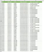
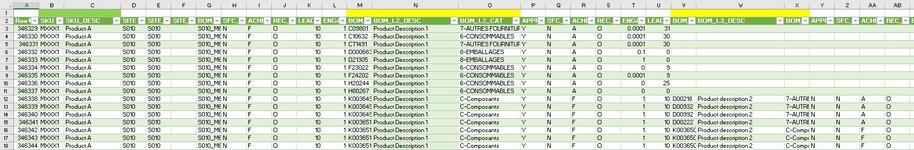
On the attached pictures are data (data tab) and the result I am looking for (desired result tab).
For a given product in column B, I want to find values in columns M, V, AE, AN, AW, BF, and BO, and paste those values in a list (along with the following 2 columns after M, V, AE, AN, etc) on a separate sheet, then remove duplicates in column C of the separate sheet.
The loop would then go through all products in the data tab in column B and do the same. I have up to 25k rows.
Thank you for your help.

 

[Domenic]

Yes, from post #9 I confirm that this is the line giving the error:View attachment 41051

View attachment 41050

That line of code should be fine, but does it help if you changed it to...

arrB = Range("B3:B" & Cells(Rows.Count, "B").End(xlUp).Row).Value

???

 

[mlepesant]

It is not clear what to do with this second and subsequent product. Does it get appended to the bottom of the first product data in the results sheets or does it replace? I have assumed appended at the bottom.

Correct. All subsequent products should then be appended to the previous ones.

It now seems to me that you want all the rows from Data moving to Results, but only those specific columns. If we then sort the data appropriately and remove duplicates (columns A & C on the Result sheet), would we have what you want?

Yes! That is exactly what I need

Could you also confirm (if the code below does not do what you want) whether those headings on the Data sheet are actually in row 2 or row 1. I am now assuming that they are actually in row 1 and you just moved them down so that you could show us with the green and yellow in row 1 of the image in post #1which columns toy wanted extracted.

Your assumption is correct. The headings in the data sheet are actually in row 1. I moved them down for the reason you are mentionning.

I am also assuming a 'Result' sheet exists and that it is empty or any data in it can be removed. Please advise details if this is not correct.

Again correct! The sheet exists. Does the code clean this sheet before it starts its routine?

I will be trying the code soon and get back to you with feedback.
Thank you very much for the time you are spending on this.

I could be way off the mark but this is what I am thinking.

Sub Get_Data_v2()
  Dim aCols As Variant
  Dim lr As Long
 
  aCols = Split("2 3 13 14 15 22 23 24 31 32 33 40 41 42 49 50 51 58 59 60 67 68 69")  '<- Cols B, C, M, N, O, V, W, X, ..., BO, BP, BQ
  Application.ScreenUpdating = False
    lr = Sheets("Data").Cells.Find(What:="*", LookIn:=xlValues, SearchOrder:=xlByRows, SearchDirection:=xlPrevious).Row
    With Sheets("Result")
      .UsedRange.ClearContents
      .Range("A1").Resize(lr, UBound(aCols) + 1).Value = Application.Index(Sheets("Data").Cells, Evaluate("row(1:" & lr & ")"), aCols)
      With .UsedRange
        .Sort Key1:=.Columns(1), Order1:=xlAscending, Key2:=.Columns(3), Order2:=xlAscending, Header:=xlYes
        .RemoveDuplicates Columns:=Array(1, 3), Header:=xlYes
      End With
    End With
  Application.ScreenUpdating = True
End Sub

 

[mlepesant]

Correct. All subsequent products should then be appended to the previous ones.

Yes! That is exactly what I need

Your assumption is correct. The headings in the data sheet are actually in row 1. I moved them down for the reason you are mentionning.

Again correct! The sheet exists. Does the code clean this sheet before it starts its routine?

I will be trying the code soon and get back to you with feedback.
Thank you very much for the time you are spending on this.

It is actually not far at all.

In the picture pasted, I highlight in yellow what the final result should look like (for space saving purpose I have grouped the columns I don't care about):

All item highlighted in yellow, belong to the product in column B.
Column V breaks down items that are in column M.
Column AE breaks down items that are in column V
Column AN breaks down items that are in column AE
Column AW breaks down items that are in column AN

So all highlighted items should then be listed in the Result sheet in the same column

Then the same process takes place for a different product in Column B, and all results should be appended to the previous ones.

 

[mlepesant]

It is not clear what to do with this second and subsequent product. Does it get appended to the bottom of the first product data in the results sheets or does it replace? I have assumed appended at the bottom.

It now seems to me that you want all the rows from Data moving to Results, but only those specific columns. If we then sort the data appropriately and remove duplicates (columns A & C on the Result sheet), would we have what you want?

Could you also confirm (if the code below does not do what you want) whether those headings on the Data sheet are actually in row 2 or row 1. I am now assuming that they are actually in row 1 and you just moved them down so that you could show us with the green and yellow in row 1 of the image in post #1which columns toy wanted extracted.

I am also assuming a 'Result' sheet exists and that it is empty or any data in it can be removed. Please advise details if this is not correct.

I could be way off the mark but this is what I am thinking.

Sub Get_Data_v2()
  Dim aCols As Variant
  Dim lr As Long
 
  aCols = Split("2 3 13 14 15 22 23 24 31 32 33 40 41 42 49 50 51 58 59 60 67 68 69")  '<- Cols B, C, M, N, O, V, W, X, ..., BO, BP, BQ
  Application.ScreenUpdating = False
    lr = Sheets("Data").Cells.Find(What:="*", LookIn:=xlValues, SearchOrder:=xlByRows, SearchDirection:=xlPrevious).Row
    With Sheets("Result")
      .UsedRange.ClearContents
      .Range("A1").Resize(lr, UBound(aCols) + 1).Value = Application.Index(Sheets("Data").Cells, Evaluate("row(1:" & lr & ")"), aCols)
      With .UsedRange
        .Sort Key1:=.Columns(1), Order1:=xlAscending, Key2:=.Columns(3), Order2:=xlAscending, Header:=xlYes
        .RemoveDuplicates Columns:=Array(1, 3), Header:=xlYes
      End With
    End With
  Application.ScreenUpdating = True
End Sub

Peter_SSs . I think I replied to myself on post #23, but you should see it?

 

[igold]

Why don't you just post your workbook to a file sharing site such DropBox with or without real information. This way we all can see what is going on.

 

[mlepesant]

Why don't you just post your workbook to a file sharing site such DropBox with or without real information. This way we all can see what is going on.

Hi igold. Let me try to add one more picture, and then if that doesn't help I will move on to sharing the file if I figure out how

From the Data on post #23, the result should look like this. The yellow highlighted items below are each unique item from column M, V, AE, AN, AW, BF, for each products in column B.

 

[Peter_SSs]

Does the code clean this sheet before it starts its routine?

My code clears anything already in the Result sheet before writing the new data into it.