VBA to select range from another sheet on drop down selection

[Bamh1]

Hello,

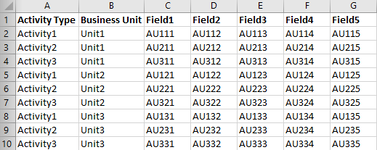
I have a master sheet that contains combinations of activity types for 3 business units, and Infront of each combination there is a row of information.

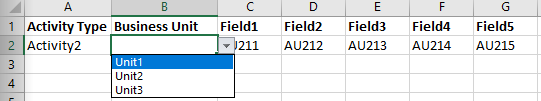
In another sheet, I have created drop down menus for the activity types (Col. A), and business units(Col. B). Upon selection of the drop down in column B, I want the corresponding row of information (range c:g) for that particular combination copied from the master sheet in front of the selection.

Could someone please help with a VBA or if there is another way to do this non programmatically.

Thank you.

Shawn

 

[kevin9999]

You should have XLOOKUP() with 2016, so the following will avoid the need for VBA. Assumes your table of data is on Sheet1 (change to suit).

Book1
	A	B	C	D	E	F	G
1	Activity Type	Business Unit	Field1	Field2	Field3	Field4	Field5
2	Activity2	Unit2	AU221	AU221	AU221	AU221	AU221
3
Sheet2

Cell Formulas
Range	Formula
C2:G2	C2	=XLOOKUP($A$2&$B$2,Sheet1!$A$2:$A$10&Sheet1!$B$2:$B$10,Sheet1!C2:C10,"")

Cells with Data Validation
Cell	Allow	Criteria
A2	List	=$I$1:$I$3
B2	List	=$J$1:$J$3

 

[kevin9999]

The data set I used in post #2 wasn't a true reflection of yours, so here's another look.

Data set (Master sheet)

xlookup.xlsx
	A	B	C	D	E	F	G
1	Activity Type	Business Unit	Field1	Field2	Field3	Field4	Field5
2	Activity1	Unit1	AU111	AU112	AU113	AU114	AU115
3	Activity2	Unit1	AU211	AU212	AU213	AU214	AU215
4	Activity3	Unit1	AU311	AU312	AU313	AU314	AU315
5	Activity1	Unit2	AU121	AU122	AU123	AU124	AU125
6	Activity2	Unit2	AU221	AU222	AU223	AU224	AU225
7	Activity3	Unit2	AU321	AU322	AU323	AU324	AU325
8	Activity1	Unit3	AU131	AU132	AU133	AU134	AU135
9	Activity2	Unit3	AU231	AU232	AU233	AU234	AU235
10	Activity3	Unit3	AU331	AU332	AU333	AU334	AU335
Sheet1

Result

xlookup.xlsx
	A	B	C	D	E	F	G
1	Activity Type	Business Unit	Field1	Field2	Field3	Field4	Field5
2	Activity2	Unit2	AU221	AU222	AU223	AU224	AU225
3
Sheet2

Cell Formulas
Range	Formula
C2:G2	C2	=XLOOKUP($A$2&$B$2,Sheet1!$A$2:$A$10&Sheet1!$B$2:$B$10,Sheet1!C2:C10,"")

Cells with Data Validation
Cell	Allow	Criteria
A2	List	=$I$1:$I$3
B2	List	=$J$1:$J$3

 

[Fluff]

You should have XLOOKUP() with 2016

Xlookup is only available in 365 & 2021.

 

[Bamh1]

The data set I used in post #2 wasn't a true reflection of yours, so here's another look.

Data set (Master sheet)

xlookup.xlsx
	A	B	C	D	E	F	G
1	Activity Type	Business Unit	Field1	Field2	Field3	Field4	Field5
2	Activity1	Unit1	AU111	AU112	AU113	AU114	AU115
3	Activity2	Unit1	AU211	AU212	AU213	AU214	AU215
4	Activity3	Unit1	AU311	AU312	AU313	AU314	AU315
5	Activity1	Unit2	AU121	AU122	AU123	AU124	AU125
6	Activity2	Unit2	AU221	AU222	AU223	AU224	AU225
7	Activity3	Unit2	AU321	AU322	AU323	AU324	AU325
8	Activity1	Unit3	AU131	AU132	AU133	AU134	AU135
9	Activity2	Unit3	AU231	AU232	AU233	AU234	AU235
10	Activity3	Unit3	AU331	AU332	AU333	AU334	AU335
Sheet1

Result

xlookup.xlsx
	A	B	C	D	E	F	G
1	Activity Type	Business Unit	Field1	Field2	Field3	Field4	Field5
2	Activity2	Unit2	AU221	AU222	AU223	AU224	AU225
3
Sheet2

Cell Formulas
Range	Formula
C2:G2	C2	=XLOOKUP($A$2&$B$2,Sheet1!$A$2:$A$10&Sheet1!$B$2:$B$10,Sheet1!C2:C10,"")

Cells with Data Validation
Cell	Allow	Criteria
A2	List	=$I$1:$I$3
B2	List	=$J$1:$J$3

Thank you so much for taking the time to review this post. Your solution works.

 

[Fluff]

Your solution works.

In that case what version of Excel are you using? 2016 does not have the XLOOKUP function.

 

[Bamh1]

In that case what version of Excel are you using? 2016 does not have the XLOOKUP function.

I do have access to excel365, and tested out the xlookup solution; however, I eventually need a VBA solution because: 1) xlookup only finds cell values and not formatting, and the reference cells are color-coded; 2) xlookup solution limits transferability of the file to the machines that don't have the latest excel version. Do you know a VBA code that could help in this situation?
Thanks

 

[Fluff]

I eventually need a VBA solution because: 1) xlookup only finds cell values and not formatting, and the reference cells are color-coded

This is the sort of thing that you should have mentioned originally.