VBA transit the formula

[Maci3j]

Hi everyone,

I would like to ask you for help.
I recorded a macro which does three things:
- column A: transits the formula,
- column A, J, K, N: colors the column names in red,
- column F, G, H, J, K, L, M, N, O: changes the format to date.


This is the macro:

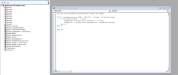
Sub OTIF()
'
' OTIF Macro
'

'
Sheets("OTIF").Select
Range("A2").Select
Application.CutCopyMode = False
Selection.AutoFill Destination:=Range("A2:A1000")
Range("A2:A1000").Select
Columns("F:O").Select
Selection.NumberFormat = "m/d/yyyy"
Range("A1,J1:K1,N1").Select
Range("N1").Activate
With Selection.Interior
.Pattern = xlSolid
.PatternColorIndex = xlAutomatic
.Color = 255
.TintAndShade = 0
.PatternTintAndShade = 0
End With
Sheets("Instructie").Select
End Sub


The issue:
I would like to adapt it so the formula in column A6 will be transited to A7 if cell B7 is not empty.
Could you please help me with it?

Thank you in advance!

 

[Zot]

This is a worksheet event triggered. So copy this code in Worksheet module (not normal module).

Any change in Range("B2:B1000") will trigger the macro. If cell (refers as Target) is not blank, the code will copy formula from 1 row above and paste.

Private Sub Worksheet_Change(ByVal Target As Range)

If Not Intersect(Range("B2", "B1000"), Target) Is Nothing Then
    If Not Len(Target) = 0 Then
        Range("A" & Target.Row).Offset(-1, 0).Copy
        Range("A" & Target.Row).PasteSpecial (xlPasteFormulas)
    End If
End If

End Sub

 

[Maci3j]

This is a worksheet event triggered. So copy this code in Worksheet module (not normal module).

Any change in Range("B2:B1000") will trigger the macro. If cell (refers as Target) is not blank, the code will copy formula from 1 row above and paste.

Private Sub Worksheet_Change(ByVal Target As Range)

If Not Intersect(Range("B2", "B1000"), Target) Is Nothing Then
    If Not Len(Target) = 0 Then
        Range("A" & Target.Row).Offset(-1, 0).Copy
        Range("A" & Target.Row).PasteSpecial (xlPasteFormulas)
    End If
End If

End Sub

unfortunately the code doesn't work.
I opened the VBA, dubble clicked on the Sheet2 (OTIF), pasted the code and saved it. Added a new value in B7 but there were no changes made in cell A7.
Did I do something wrong?

 

[Maci3j]

This is a worksheet event triggered. So copy this code in Worksheet module (not normal module).

Any change in Range("B2:B1000") will trigger the macro. If cell (refers as Target) is not blank, the code will copy formula from 1 row above and paste.

Private Sub Worksheet_Change(ByVal Target As Range)

If Not Intersect(Range("B2", "B1000"), Target) Is Nothing Then
    If Not Len(Target) = 0 Then
        Range("A" & Target.Row).Offset(-1, 0).Copy
        Range("A" & Target.Row).PasteSpecial (xlPasteFormulas)
    End If
End If

End Sub

I made a mistake in the selection.
@Zot thank you very much! the code works great!!

 

[Maci3j]

ok. I tried it again and the formula works.
However, the formula in column A only transits 4 rows lower.

 

[Zot]

ok. I tried it again and the formula works.
However, the formula in column A only transits 4 rows lower.

I don't understand what you meant by 4 rows lower.

How do you enter data in column B? The macro is triggered whenever you enter data in column B. Do you copy a range and paste?

It would be help ful if you can use XL2BB to capture the sample above and paste here. The XL2BB is a great tool that will preserve the formula and etc. into pasted sample. This was those who are helping can immediately try possible solution. Most will hesitate to re-type data and just pass the question

 

[Maci3j]

Yes exactly. The formula in column A appears only when I enter the data manually in columns B and D (D is logical as the formula in column A is based on column D) but doesn't wont with copy and paste.

OTIF sjabloon 1111 - Copy - Copy.xlsm
	A	B	C	D	E	F	G	H	I	J
1	%key_purchase_order	0VENDOR.Vendor Name	%key_shopping_cart	%key_purchase_order	%key_goods_receipts	SC creation date	SC start date	SC end date	PO item creation date	PO Start date
2	2100148353/1	ERIKS NV	1001522764|0000000001	2100148353|0000000001	8001222133|0000000001|2020	22/04/2019	22/04/2019	22/04/2019	25/02/2020	25/02/2020
3	2100146909/1	ERIKS NV	1001600475|0000000001	2100146909|0000000001	8001263609|0000000001|2020	19/09/2019	19/09/2019	19/09/2019	16/01/2020	16/01/2020
4	3300434175/1	ERIKS NV	1001622695|0000000001	3300434175|0000000001	8001229447|0000000001|2020	25/10/2019	25/10/2019	28/10/2019	15/01/2020	15/01/2020
5	2100146512/1	ERIKS NV	1001649579|0000000001	2100146512|0000000001	8001221036|0000000001|2020	12/12/2019	12/12/2019	12/12/2019	8/01/2020	8/01/2020
6	3100115453/1	ERIKS NV	1001656213|0000000001	3100115453|0000000001	8001199586|0000000001|2020	31/12/2019	31/12/2019	31/12/2019	3/01/2020	3/01/2020
7	3100115453/2	ERIKS NV	1001656213|0000000002	3100115453|0000000002	8001200537|0000000002|2020	31/12/2019	31/12/2019	31/12/2019	3/01/2020	3/01/2020
8	3100115453/3	ERIKS NV	1001656213|0000000003	3100115453|0000000003	8001200537|0000000003|2020	31/12/2019	31/12/2019	31/12/2019	3/01/2020	3/01/2020
9	2100146347/1	ERIKS NV	1001656359|0000000001	2100146347|0000000001	8001199067|0000000001|2020	2/01/2020	2/01/2020	2/01/2020	2/01/2020	2/01/2020
10	2100146336/1	ERIKS NV	1001656388|0000000001	2100146336|0000000001	8001207142|0000000001|2020	2/01/2020	2/01/2020	2/01/2020	2/01/2020	2/01/2020
11	2100146336/2	ERIKS NV	1001656389|0000000001	2100146336|0000000002	8001200335|0000000002|2020	2/01/2020	2/01/2020	2/01/2020	2/01/2020	2/01/2020
12	2100146336/3	ERIKS NV	1001656394|0000000001	2100146336|0000000003	8001199717|0000000003|2020	2/01/2020	2/01/2020	2/01/2020	2/01/2020	2/01/2020
13
14
15
16
17
18
19
20
21
OTIF

Cell Formulas
Range	Formula
A2:A12	A2	=IF(D2="","",LEFT(D2&"|"&D2,(FIND("|",D2&"|"&D2,1)-1))&"/"&CONVERT(RIGHT(D2&"|"&D2,(FIND("|",D2&"|"&D2,1)-1)),"m","m"))

 

[Maci3j]

In the mean time I thought about a better and more efficient solution.
The macro should do as follow: transit the formula from A2 below till the first empty cell in column B.

Could you please help me with it?
Thank you in advance

 

[Zot]

In the mean time I thought about a better and more efficient solution.
The macro should do as follow: transit the formula from A2 below till the first empty cell in column B.

Could you please help me with it?
Thank you in advance

My understanding is:
For current code, when enter data in column B, the formula in column A will be copied from a row above.
Now you wanted formula in column A to be copied additional row ahead of the row in column B you have just entered data.
Something like this:

Private Sub Worksheet_Change(ByVal Target As Range)

If Not Intersect(Range("B2", "B1000"), Target) Is Nothing Then
    If Not Len(Target) = 0 Then
        Range("A" & Target.Row).Offset(-1, 0).Copy
        Range(Range("A" & Target.Row), Range("A" & Target.Row).Offset(1)).PasteSpecial (xlPasteFormulas)
        Target.Select
        Application.CutCopyMode = False
    End If
End If

End Sub

 

[Maci3j]

yes it works.
many thanks!!