Need some help here! Two part question here possibly. I am not very efficient with excel yet so please bear with me!
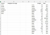
I hope the sample file link works, if not I attached an image where I combined sheet 1 and 2 into one to show an idea of what I am working with.
SAMPLE FILE
1. I need to find the weighted averages for multiple lines. I know to use the =SUMPRODUCT formula /SUM however, the issue I am having is, there are over 2,000 lines.
The only way I know how to do this is to enter the formula manually each time for each group of the same names. And that would take FOREVER to complete. I know there has to be a formula or way where it can find all the matching names, take the weights and rates and provide me the average weight! In the sample file I have more simplified than what I am working with, again I have a sheet with 2,000+ rows.
Is there an easy way to find the weighted average easily with a formula that can automatically find all the lines with the same name, then take the weight and rate and give me the weighted average?
2. If above is possible, then I could just simply create a pivot table and then vlookup the weighted averages. If not, then is there a way to vlookup the names, then provide me with the weighted average going off the weights and rates?
Thank you so much!