vlookup - font color

[haitham1984]

Hello All,

I am writing questions for a quiz and within each cell of that column (Questions Column), I am manually writing text with different font colors. The next 4 columns are the multiple choice answers for the question on the same row, which also can have different font colors. example:

Columns: A B C D E
What is the capital city of France.....Paris.....London.....Berlin.....Rome

I then use vlookup on another column (say column G to K) to arrange the questions in a pre-specified order. The Problem is that when I use vlookup the cells lose the font colors I used and also sub/superscripts for certain questions. Any ideas how to solve this problem please.

Thanks All,

 

[Yongle]

You have hit an Excel limitation
Individual characters cannot be coloured in cells containing formulas

 

[Peter_SSs]

.. but you could use a macro to copy/paste the values to retain their colour. Would need more detail about layout and sample data and how/when the rearrangement of order is to take place.

 

[haitham1984]

.. but you could use a macro to copy/paste the values to retain their colour. Would need more detail about layout and sample data and how/when the rearrangement of order is to take place.

Hello Peter_SSs,

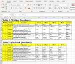
Thanks for your reply, I have attached an image of a sample of my data (since I can't upload a sample excel file here, correct? sorry Im kinda new here). Just a quick explanation: Table 1 (on the top) is roughly 2000 rows in height and it is where i enter the questions one after the other in no particular order. Table 2 (bottom) (where all formatting is lost: font colour, sub/superscripts) arranges the questions from Easy to Hard. Hope this helps, and thanks again for your effots.

Regards,

PS: Just incase you need it, the formula in cell C13 is:
=VLOOKUP(B13,$B$3:$H$9,2,FALSE)

and the formula for cell B13 is:
=IF(B12="Serial","Easy1",IF(COUNTIF($B12:B$13,"*Easy*")<COUNTIF($H$3:$H$9,"Easy"),CONCATENATE("Easy",COUNTIF($B12:B$13,"*Easy*")+1),IF(COUNTIF($B12:B$13,"*Medium*")<COUNTIF($H$3:$H$9,"Medium"),CONCATENATE("Medium",COUNTIF($B12:B$13,"*Medium*")+1),IF(COUNTIF($B12:B$13,"*Hard*")<COUNTIF($H$3:$H$9,"Hard"),CONCATENATE("Hard",COUNTIF($B12:B$13,"*Hard*")+1),"Error"))))

 

[Peter_SSs]

Any chance you could upload that small sample file to Dropbox or OneDrive etc and provide a shared link here? Even for that small sample it would be a lot of manual typing and colouring to set up to test.

Are Easy, medium & Hard the only 3 levels?

How is B3:B9 populated? Manually? Formula?

Do you really need column B in either table? If we could just get the list with all Easy first then all medium second and all Hard last, would that do? It isn't a problem to have that column, I was just thinking that you possibly only had it for your VLOOKUP (which didn't work).

I also suggest that you update your Account details (click your user name at the top right of the forum) so helpers always know what Excel version(s) & platform(s) you are using as the best solution often varies by version. (Don’t forget to scroll down & ‘Save’)

 

[haitham1984]

Any chance you could upload that small sample file to Dropbox or OneDrive etc and provide a shared link here? Even for that small sample it would be a lot of manual typing and colouring to set up to test.

Are Easy, medium & Hard the only 3 levels?

How is B3:B9 populated? Manually? Formula?

Do you really need column B in either table? If we could just get the list with all Easy first then all medium second and all Hard last, would that do? It isn't a problem to have that column, I was just thinking that you possibly only had it for your VLOOKUP (which didn't work).

I also suggest that you update your Account details (click your user name at the top right of the forum) so helpers always know what Excel version(s) & platform(s) you are using as the best solution often varies by version. (Don’t forget to scroll down & ‘Save’)

Here is a link to the file: sample data.xlsx

Yes, it's a lot of work.

Yes, there are only 3 levels, and B3:B9 are populated automatically. Yes I need column B because the actual file uses it for another reason also.

Thanks again.

 

[Peter_SSs]

Thanks for the file link.

B3:B9 are populated automatically.

Firstly, a much simpler formula for column B would be this in B2 and copied down
=H2&COUNTIF(H$2:H2,H2)

Assuming data in columns A:H and nothing in columns J:Q, try this with a copy of your workbook. Post back if you need help with implementation.

Sub Rearrange()
  Dim lngCalc As Long, lngLastRow As Long, i As Long
 
  Const sSortOrder As String = ",Easy,Medium,Hard"
 
  Application.ScreenUpdating = False
  lngCalc = Application.Calculation
  Application.Calculation = xlCalculationManual
  lngLastRow = Range("A" & Rows.Count).End(xlUp).Row
  For i = 1 To 8
    Columns(i).Offset(, 9).ColumnWidth = Columns(i).ColumnWidth
  Next i
  Range("A1:H" & lngLastRow).Copy Destination:=Range("J1")
  With Range("K2:K" & lngLastRow)
    .Value = .Value
  End With
  ActiveSheet.Sort.SortFields.Clear
  ActiveSheet.Sort.SortFields.Add2 Key:=Columns("Q"), Order:=xlAscending, CustomOrder:=sSortOrder
  With ActiveSheet.Sort
    .SetRange Range("K1:Q" & lngLastRow)
    .Header = xlYes
    .Orientation = xlTopToBottom
    .Apply
  End With
  Columns("Q").Delete
  Application.Calculation = lngCalc
  Application.ScreenUpdating = True
End Sub

 

[haitham1984]

Thanks for the file link.

Firstly, a much simpler formula for column B would be this in B2 and copied down
=H2&COUNTIF(H$2:H2,H2)

Assuming data in columns A:H and nothing in columns J:Q, try this with a copy of your workbook. Post back if you need help with implementation.

Sub Rearrange()
  Dim lngCalc As Long, lngLastRow As Long, i As Long

  Const sSortOrder As String = ",Easy,Medium,Hard"

  Application.ScreenUpdating = False
  lngCalc = Application.Calculation
  Application.Calculation = xlCalculationManual
  lngLastRow = Range("A" & Rows.Count).End(xlUp).Row
  For i = 1 To 8
    Columns(i).Offset(, 9).ColumnWidth = Columns(i).ColumnWidth
  Next i
  Range("A1:H" & lngLastRow).Copy Destination:=Range("J1")
  With Range("K2:K" & lngLastRow)
    .Value = .Value
  End With
  ActiveSheet.Sort.SortFields.Clear
  ActiveSheet.Sort.SortFields.Add2 Key:=Columns("Q"), Order:=xlAscending, CustomOrder:=sSortOrder
  With ActiveSheet.Sort
    .SetRange Range("K1:Q" & lngLastRow)
    .Header = xlYes
    .Orientation = xlTopToBottom
    .Apply
  End With
  Columns("Q").Delete
  Application.Calculation = lngCalc
  Application.ScreenUpdating = True
End Sub

Thanks Peter...it works fine but there is a problem. When the questions are transferred to the table on the right, I lost all the vlookup formulas, and everything became text. The reason why i still need the formulas is because each level of questions (Easy,Medium,Hard) has roughly 600 questions per level, and i ordered them randomly which requires the use of the vlookup formula. Is there are a way to modify the macro to leave the formulas of each cells intact in the table on the right?

Sorry if i didn't mention this earlier and thanks again for your effort.

 

[Peter_SSs]

No, as Yongle correctly stated earlier

Individual characters cannot be coloured in cells containing formulas

How/where are you ordering them randomly?

Presumably that is somehow in columns A:H. If you re-order them there in a different random order, can't you just run the macro again to get the new order in columns J:P?

 

[haitham1984]

Sorry for the Delay in Replying,

Actually that wont work, guess I will have to do it manually. But that's okay, shouldn't take too long to do.

Thanks again for all your help, and take care