Vlookup help, comparing list

[Full Spool]

Hello,

I am having issues comparing 2 rows with vlookup. My issue is some of my numbers have a "-5" after a series of numbers. Vlookup thinks the numbers
don't exist in my reference data. I don't know how to fix my formula to ignore the "-5" and look at the numbers before so it can draw
a correct comparison.

My formula below "
=VLOOKUP(D2,Mapping!$A$2:$A$61,1,FALSE)

You can see when the -5 is in the Billing Tab and on the Mapping Tab in excel it works. However once the -5 is missing in the billing tab
it no longer correlates.

Thanks in advance for any help or direction provided.

 

[AhoyNC]

Will there always be 5 numbers before the dash as in your example?

 

[Full Spool]

Will there always be 5 numbers before the dash as in your example?

no, sometimes there is something like xx1251, or "no meter" text with no numbers at all.

 

[AhoyNC]

I have not been able to figure out a reliable way to handle your second request. Hopefully someone else may be able to help.

 

[Full Spool]

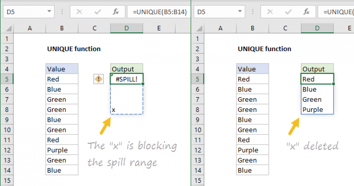
Thanks for the help @AhoyNC , can you tell me what #SPILL! means and how to fix it? 17269-5 is in the mapping tab ?

 

[AhoyNC]

See attached link on #SPILL.

How to fix the #SPILL! error

Most often, a #SPILL! error occurs when a spill range is blocked by something on the worksheet, and the solution is to clear the spill range of any obstructing data. However, a #SPILL! error can have other causes as well. Read below for details.

exceljet.net

 

[Full Spool]

@AhoyNC How can I rewrite the formula to compare the mapping tab values in column A to see if they match the values in column A in the billing tab? Basically the inverse of what
your original formula is doing.

=FILTER('Mapping tab'!$A$2:$A$200,ISNUMBER(SEARCH(A2,'Mapping tab'!$A$2:$A$200)),"No Match")

 

[AhoyNC]

Post some examples of the data in billing tab A that you want to match in column A of the mapping tab. As you are aware the issue is with the inconsistent data between the 2 tabs.

 

[Full Spool]

Billing Tab

Mapping Tab

 

[AhoyNC]

Maybe something like this.
Just be aware that the way SEARCH works and depending on your data it could show a natch when there isn't one.

Book (4).xlsx
	A	B	C
1	Billi		Meterc
2	11252		11252-8
3	11310		11310-5
4	11399		11399-5
5	11661		11661-5
6	11981		11981-5
7	12514		12514-5
8	12640		12640-5
9	12706		12706-5
10	12709		12709-5
11	16477		16477-0
12	16480		16480-0
13	16500		16500-0
14	17094		17094-5
15	17130		17130-0
16	17135		17135-0
17	17292		17292-0
18	17299		17299-0
19	17859		17859-0
20	18215		18215-0
21	16254	No Match	22025-55
Sheet1

Cell Formulas
Range	Formula
B2:B21	B2	=IF(ISNUMBER(SEARCH($A2,$C$2:$C$21)),"","No Match")

 

[Full Spool]

Maybe something like this.
Just be aware that the way SEARCH works and depending on your data it could show a natch when there isn't one.

Book (4).xlsx
	A	B	C
1	Billi		Meterc
2	11252		11252-8
3	11310		11310-5
4	11399		11399-5
5	11661		11661-5
6	11981		11981-5
7	12514		12514-5
8	12640		12640-5
9	12706		12706-5
10	12709		12709-5
11	16477		16477-0
12	16480		16480-0
13	16500		16500-0
14	17094		17094-5
15	17130		17130-0
16	17135		17135-0
17	17292		17292-0
18	17299		17299-0
19	17859		17859-0
20	18215		18215-0
21	16254	No Match	22025-55
Sheet1

Cell Formulas
Range	Formula
B2:B21	B2	=IF(ISNUMBER(SEARCH($A2,$C$2:$C$21)),"","No Match")

I tried the formula but I am getting no match.