Vlookup Help

[tomehta]

Hello
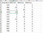
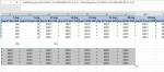
In attached excel screen shots, in Col I (sheet 1), I want Col C value (from sheet 2), similarly in Col P (sheet 1) want Col D value( from Sheet 2). I am trying with variations of Columns function but not able to crack. I want to create formula in col B sheet 1 and drag it. I dont want to manually update formula in Col I and Col P ( and hence forth). Any help will be greatly appreciated.

 

[tomehta]

Thanks for pointing it out..this will be wrong ..

basically I am skipping 6 columns from AppView reference sheet, but at the same time I am dragging in alternate columns in variance columns. Any pointer will be greatly appreciated.

 

[tomehta]

Something like below is the requirement, any suggestion would be of great help

 

[jasonb75]

I hadn't realised exactly what you meant before, the proverbial penny has dropped now, enter the first formula into B2, the second into C2, then select both cells and drag right as a pair.

=INDEX(AppView!$E2:$DN2,,COLUMNS($B2:B2)*8-8+1) - INDEX(AppView!$I2:$DN2,,COLUMNS($B2:B2)*8-8+1)
=INDEX(AppView!$F2:$DN2,,COLUMNS($C2:C2)*8-8+1) - INDEX(AppView!$J2:$DN2,,COLUMNS($C2:C2)*8-8+1)

 

[tomehta]

Using the step of 8, results are not correct.

 

[jasonb75]

Change 8-8 to 4-4 in both parts of the formula.

Because you're dragging the formulas as a pair the increase needs to be halved, I forgot to allow for this.

 

[tomehta]

Something is missing sir..

--
Another issue is
After dragging for some cols, its started giving Ref error. Thats the case with what ever steps I choose...

 

[jasonb75]

I miscounted the number of columns, easily done when working with screen captures.

Going back, it looks like your initial effort of using 3.5 was correct, you just needed the paired formula method to make it work.

If you remember what I said about the irregular pattern when you drag a fraction / decimal. That is normally the case, but by dragging in pairs it will even itself out (3.5 in each formula still totals to 7).

For future questions / posts, please use XL2BB (see link below) to post your samples so that we can copy them to excel and test formulas before posting them.

XL2BB - Excel Range to BBCode

Excel 'mini-sheet' in messages - XL2BB Although experts prefer to read your description and question instead of working in your actual file to solve your problem, there are times that it is difficult to explain an issue without providing actual...

www.mrexcel.com

 

[tomehta]

Thanks for quick response, 3.5 was working fine till but after some cells it started giving error. I checked the columns its calculated correctly and reference sheet has data corresponding to columns reference.

Another issue is
After dragging for some cols, its started giving Ref error. Thats the case with what ever steps I choose...

I was getting the impression since I used 3.5 , excel is messing it up. but its case even we use 4 or 8.

Reference Excel,

Regarding XLBB, I am using office 365 and seems my organization has'nt installed XLBB add in. I will dig more.

 

[tomehta]

well I spoke to early.

Forecast DASH v12.0.xlsx
	AD	AE	AF	AG	AH	AI	AJ
1	31-Jul	31-Jul	7-Aug	7-Aug	14-Aug	14-Aug	21-Aug
2	Jul-31 BAU VAR	Jul-31 Project VAR	Aug-07 BAU VAR	Aug-07 Project VAR	Aug-14 BAU VAR	Aug-14 Project VAR	Aug-21 BAU VAR
3	560	70	560	70	#REF!	#REF!	#REF!
4	120	15	120	15	#REF!	#REF!	#REF!
5	160	20	160	20	#REF!	#REF!	#REF!
6	400	50	400	50	#REF!	#REF!	#REF!
7	120	15	120	15	#REF!	#REF!	#REF!
8
9	99		106		113
Variance

Cell Formulas
Range	Formula
AD1:AJ1	AD1	=AB1+7
AD2,AF2,AH2,AJ2	AD2	=CONCAT(TEXT(AD1, "MMM-DD")," BAU VAR")
AE2,AG2,AI2	AE2	=CONCAT(TEXT(AE1,"MMM-DD")," Project VAR")
AD3:AD7,AF3:AF7,AH3:AH7,AJ3:AJ7	AD3	=INDEX(AppView!$E2:$DN2,,COLUMNS($E2:AG2)*3.5-3.5+1) - INDEX(AppView!$I2:$DN2,,COLUMNS($I2:AK2)*3.5-3.5+1)
AE3:AE7,AG3:AG7,AI3:AI7	AE3	=INDEX(AppView!$F2:$DN2,,COLUMNS($F2:AH2)*3.5-3.5+1) - INDEX(AppView!$J2:$DN2,,COLUMNS($J2:AL2)*3.5-3.5+1)
AD9,AH9,AF9	AD9	=COLUMNS($E2:AG2)*3.5-3.5+1

 

[jasonb75]

Second part of your formula is causing the error,

=INDEX($E2:$DN2,,COLUMNS($B2:B2)*3.5-3.5+1)-INDEX($I2:$DN2,,COLUMNS($I2:AO2)*3.5-3.5+1)

BAU Actl Aug-14 is going to be in $DQ12 which is outside of the range that you used in the formula

Enter the first one in B2, the second in C2, then select and drag as a pair. Do not change anything

=INDEX(2:2,,COLUMNS($B2:B2)*3.5-3.5+5)-INDEX(2:2,,COLUMNS($B2:B2)*3.5-3.5+9)
=INDEX(2:2,,COLUMNS($C2:C2)*3.5-3.5+6)-INDEX(2:2,,COLUMNS($C2:C2)*3.5-3.5+10)