vlookup in column and row

[mtagliaferri]

I am wondering if vlookup is the right approach for my issue, if so any help is greatly appreciated!

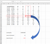
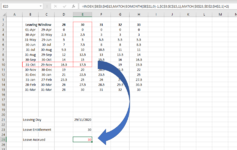
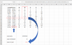
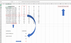
I have a table which dictates how many days of leave a person has accrued depending on the leaving date and their annual entitlement, in the attachment I have a leaving date of 15/09/20 (E21) and the entitlement per year of 31 days (E23) I would like to return the correct number 15.5 in cell E25.
I have formatted the leaving window to display the date as dd-mmm however in the cell it display also the yyyy, I would like that to be a generic dd-mmm however I am conscious that the leaving date entered in E21 is a full date including the year.

Any ideas

 

[maabadi]

Use this:

=INDEX($B$3:$I$16,MATCH(EOMONTH($C$19,0)-1,$C$3:$C$16,1),MATCH($C$21,$D$2:$I$2,1)+2)

1. $B$3:$I$16 Replace it with your Total Range Data Address
2. $C$19 Replace it with your Date Criteria Address
3. $C$3:$C$16 Replace it with your 2nd column of Date Range Address. I use this formula for 2nd column of Date based of first : =EOMONTH(B4,1)-1
4. $C$21 Replace it with your Number Criteria Address
5. $D$2:$I$2 Replace it with your Header Number Range Address

 

[mtagliaferri]

Use this:

=INDEX($B$3:$I$16,MATCH(EOMONTH($C$19,0)-1,$C$3:$C$16,1),MATCH($C$21,$D$2:$I$2,1)+2)

1. $B$3:$I$16 Replace it with your Total Range Data Address
2. $C$19 Replace it with your Date Criteria Address
3. $C$3:$C$16 Replace it with your 2nd column of Date Range Address. I use this formula for 2nd column of Date based of first : =EOMONTH(B4,1)-1
4. $C$21 Replace it with your Number Criteria Address
5. $D$2:$I$2 Replace it with your Header Number Range Address

Thanks maabadi, I am definitely getting closer to what I was looking for and was wrongly thinking I needed a vlookup.
I have applied the formula has you mentioned but I am getting some wrong data:
E.G. based on 30 day entitlement column if I enter:
30/04/20 I get a result of 0 but I should get 2.5 as it falls in the range 30-Apr / 30-May (B4:C4)
31/05/20 I get a result of 2.5 but I should get 5 as it falls in the range 31-May / 29-Jun (B5:C5)
it all works fine till I enter any dates from November onwards and then all results are 30 no matter what date you enter after 01/11

 

[maabadi]

For Me, Work Fine. One Other thing.
1. At Cell B4 write:

=C3+1

2.At Cell C4 should be written:

=EOMONTH(B4,1)-1

then Select Both and Drag them down.

& Check Your Number Formats Also.

 

[mtagliaferri]

Thanks again for your patience, I am getting there but there is one more error, the start date in column B does not seem to return the correct result.
E.G. based on 30 day entitlement column if I enter:
30/09/20 I get a result of 12.5, I should get 15
31/10/20 I get 15 I should get 17.5

I have amended entered the formulas as your last post but I have the issue in C15 it should be 31-Mar where it would trigger the full leave allowance.

 

[maabadi]

Change formula to this:

=INDEX($B$3:$H$15,MATCH(EOMONTH($E$21+1,0)-1,$C$3:$C$15,1),MATCH($E$21,$D$2:$H$2,1)+2)

 

[maabadi]

And Change that Cell manually to 31-Mar.

 

[maabadi]

Finally I Find this solution. First Change that Cell manually to 31-Mar. Then Use:

=INDEX($B$3:$H$15,IF(DAY($C$15)&MONTH($C$15)=DAY($E$21)&MONTH($E$21),13,IF(MONTH($E$21+1)<=3,MONTH($E$21+1)+9,MONTH($E$21+1)-3)),MATCH($E$23,$D$2:$H$2,1)+2)

 

[mtagliaferri]

Thanks so much this is spot on what I needed!! I tested various options and it all seems to return the correct result!

I am conscious that we will be moving to 2021 and therefore I would have to amend B3 and C3 to reflect 2021 year, I therefore set a dynamic year to change accordingly to the current year; I have set as a reference M2 and N2 to as starting dates 01 April 2019 and 29 April 2019 and used the below formula for
B3:

=DATE(YEAR(TODAY()),MONTH(M2),DAY(M2))

C3:

=DATE(YEAR(TODAY()),MONTH(N2),DAY(N2))

This works fine but is there a way to avoid having reference cells for the year and just place the formula in B3 and C3, I have tehe below formula that return the 1st day of the month and the 29th as following:
1st day:

=DATE(YEAR(TODAY()),MONTH(7),DAY(1))

29th day:

=DATE(YEAR(TODAY()),MONTH(4),DAY(29))

Which ever number I place in the month section of the code it still return January, how do I return April in the formula? "=DATE(YEAR(TODAY()),MONTH(April),DAY(29))"

 

[maabadi]

Formula also work for 2021. About Formula at column B & C , Please only Input data manually at B3 and Use formula I writed at Post #4.
About Date formula, for Month & Day , you should input as number always. and You should write: "=Date(2020,4,29)" otherwise if you use month and year function, you needed serial number for them. also you can enter only month and day values at source cells. and if you want input as numbers, you should find days from 1-jan to your specific day to return month correctly, for example 92 to 121 return April:
31 (jan) + 29 (feb) + 31 (mar) = 91 & 31 (jan) + 29 (feb) + 31 (mar) + 30 (Apr) = 121