Vlookup, Index, Match

[PhebySamuel]

Hi All,

I need some help creating a formula. So I’ll explain the data in my document and then I’ll explain what I want out of my formula!

My document has several tabs. The first tab is the summary tab where the formulas will go. All the other tabs will feed into the formulas in the first tab. So, all the other tabs are certain tests that I am performing and getting a pass or fail result based on some criteria that I have created.

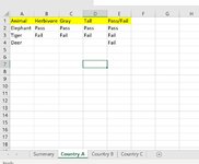
For example: tab #2 has lets say column A that has a list of things/places/animals etc. Columns B through E in tab #2 are 4 different criteria for the items in column A. If they pass the 4 criteria, each of the cells i.e. B1 C1 D1 and E1 will have Pass, and similarly if they fail one of the criteria then that cell will have Fail listed in it. Now column F is the summary result column for just this tab. Which means if in row1, if there is even one Fail among the 4 criteria, then F1 will show Fail as a summary for that particular item. F1 can only show pass if all the 4 criteria are a pass.

If I do not have information to test the 4 criteria, then those 4 boxes will be blank

I have multiple such testing tabs starting from tab#2! Each tab lets say represents a country.

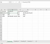
Now, going back to the very first tab which is the summary tab for all tabs is very all the formulas are going to be. In this tab, I have listed out all the items such as things/animals in column A and I have listed out the countries (that start from tab #2) in rows B1 through let’s say G1. Basically created a table outline, if that makes sense.

I want to create a formula, that will lookup the items listed in column A of tab 1 in the specific country’s tab starting from tab #2 in its Column A and once it finds that item in tab #2, then it will look across the row to look for the 4 criteria results. If the 4 criteria boxes are filled out, then it will give me the result listed in column F for that specific item. If the 4 criteria boxes are blank, then it will return “No Result Found” message.

 

[C Moore]

I'd recommend formatting the data as tables on tab 2+. Tab 2 would have Table_Nigeria.
Column F, =IF(SUMPRODUCT(ISTEXT(Table_Nigeria[@[tall]:[gray]])-1)<>0,"No Result Found",AND(Table_Nigeria[@[tall]:[gray]]="Pass"))

SUMPRODUCT/ISTEXT checks for something in the cell, AND checks that they all match.

I couldn't quite follow the tab 1 setup, but this formula will look for the animal and country.
On tab 1 the formula would be =XLOOKUP(A1,INDIRECT("Table_"&B1&"[animal]"),INDIRECT("Table_"&B1&"[Pass?]"),"Country missing animal",0)

Using indirect allows a variable assuming you name all the tables, Table_Country.

 

[PhebySamuel]

I'd recommend formatting the data as tables on tab 2+. Tab 2 would have Table_Nigeria.
Column F, =IF(SUMPRODUCT(ISTEXT(Table_Nigeria[@[tall]:[gray]])-1)<>0,"No Result Found",AND(Table_Nigeria[@[tall]:[gray]]="Pass"))
View attachment 47367
SUMPRODUCT/ISTEXT checks for something in the cell, AND checks that they all match.

I couldn't quite follow the tab 1 setup, but this formula will look for the animal and country.
On tab 1 the formula would be =XLOOKUP(A1,INDIRECT("Table_"&B1&"[animal]"),INDIRECT("Table_"&B1&"[Pass?]"),"Country missing animal",0)
View attachment 47368
Using indirect allows a variable assuming you name all the tables, Table_Country.

Thank you so much for your response. I have attached some screenshots to explain my problem better.

I'd recommend formatting the data as tables on tab 2+. Tab 2 would have Table_Nigeria.
Column F, =IF(SUMPRODUCT(ISTEXT(Table_Nigeria[@[tall]:[gray]])-1)<>0,"No Result Found",AND(Table_Nigeria[@[tall]:[gray]]="Pass"))
View attachment 47367
SUMPRODUCT/ISTEXT checks for something in the cell, AND checks that they all match.

I couldn't quite follow the tab 1 setup, but this formula will look for the animal and country.
On tab 1 the formula would be =XLOOKUP(A1,INDIRECT("Table_"&B1&"[animal]"),INDIRECT("Table_"&B1&"[Pass?]"),"Country missing animal",0)
View attachment 47368
Using indirect allows a variable assuming you name all the tables, Table_Country.

Thank you so much for your response. I have attached some screenshots to explain my question better.

 

[jasonb75]

In B2, fill right and down as needed.

=VLOOKUP($A2,INDIRECT("'"&B$1&"'!A2:E100"),5,0)

 

[PhebySamuel]

In B2, fill right and down as needed.

=VLOOKUP($A2,INDIRECT("'"&B$1&"'!A2:E100"),5,0)

Hi thanks for your response. I have not yet used the indirect function before but one thing I forgot to mention is that the order of the items listed i.e. in this case animals can be different in all the tabs! So in the summary tab, it can be tiger, deer, elephant, in the country A tab, it can be deer, tiger, elephant. So, I want my formula to look up the item regardless of which order or is in and THEN check it’s corresponding rows for passes and fails. Does the indirect function do that? I haven’t tried the formula you guys provided, but just wanted to check before I worked on my spreadsheet.

Thanks a lot for both of your help!

 

[jasonb75]

The only thing that indirect does is take the sheet name from the top row, the vlookup part will work the same as it would without indirect, it will find the animal name in column A then tell you if it is pass or fail.

As far as I can see the formula will do what you want, but I did only base it on the screen captures in your second post and the last paragraph of the first one. The description that you gave initially was a bit confusing so there may be details that I missed.

 

[PhebySamuel]

The only thing that indirect does is take the sheet name from the top row, the vlookup part will work the same as it would without indirect, it will find the animal name in column A then tell you if it is pass or fail.

As far as I can see the formula will do what you want, but I did only base it on the screen captures in your second post and the last paragraph of the first one. The description that you gave initially was a bit confusing so there may be details that I missed.

Hi,

So I tried the indirect formula that both of you suggested, but it is not doing what I want it to do. Let me see if I can explain my question a little better.

So, as I mentioned every tab starting from tab #2 have different animal or whatever names. So, let’s say for my project, I’m working with 10 animal names. Some of these tabs may not have all of those 10 names and some tabs may have all of those names listed in its column A.

For my project, I am testing 4 different criteria for each of these animals. These criteria will be tested in columns B through E with a pass or fail result, starting from tab #2. And then, in column F, I will have the final result for this animal i.e. if all of the 4 criteria are a Pass, then in column of tabs #2, 3, 4, etc will be a Pass. If one of those four criteria is a Fail, then the final result in column F, will be a Fail.

Now, there can be instances where I do not have any information about a particular animal to test the four criteria. In those cases, the four columns from B through E in tabs #2 onwards will be blank.

Now, in tab #1, which is the Summary tab, it will have all the 10 animal names listed in column A, regardless of whether it is there in one of the other tabs or not. Why? Because this is the summary tab and I need to know the result of these animals listed in each of the tabs which lets represents different countries. So, I want to know the testing result of a kangaroo in Australia and also a kangaroo in India. Based on that scenario, the testing results for kangaroo in the India tab would be all blank in columns B through E because I have no information available of kangaroos in India.

What I want my formula to do is, ask it to lookup an animal listed in the summary tab… look it up in let’s say tab #4, if it finds the specific animal from the Summary tab in tab #4, THEN I want it to look across that row in tab #4 and look at the four columns from B through E. If those cells are not blank <>“” , then give me the value listed in column F which is the final results column which could be a pass or fail depending on the results in cells B through E.

Now, when my formula is initially looking at cells B through E to check if it is not blank and sees that it is Blank, THEN I want it to say “No Results Found” instead of looking in column F. So, for the Kangaroo in the India tab, my formula should first look for the word Kangaroo which could be on ANY row (I don’t want to tell the formula which row it is in). Once my formula finds the kangaroo in the India tab, then it will look at the corresponding cells B through E. When it sees that it is blank, it will give me “No Results Found” message in the summary tab next to where kangaroo is listed under India column.

Basically, I don’t want to specific in the formula which cell # the kangaroo is listed on in each of the country tabs. I want my formula to figure it out! Because kangaroo can be probably listed on row1 in Australia tab and in row7 in India tab and in row 20 in the Nigeria tab!

Long story short, I want it to do the following things:

1) find the animal in each tab.
2) if it finds the animal, then look at the four results cells.
3) if the four results cell is not blank, then tell me the final result from column F.
4) if the four results cell is blank, then just tell me “No results found”.

5) Now, there can also be an instance where the animal is not even listed in one of the country tabs. For example, kangaroo may not be listed in the Canada tab. Then, in that case give me the “Animal not found” result.

I hope that makes better sense of what I want my formula to do.

Any help would be highly appreciated because I am losing my mind trying to make this work!

 

[jasonb75]

it is not doing what I want it to do

I had simplified the formula and not allowed for errors (No results found) although inconsistency in your examples is not helping, in your screen capture the result to return was in column E, you now say it is in column F.
I've allowed for 100 rows of data in each sheet, if there are more then you will need to increase the range. I've avoided using entire columns due to the necessity of INDIRECT making the formula highly inefficient.

=IFERROR(VLOOKUP($A2,INDIRECT("'"&B$1&"'!A2:F100"),6,0)&"","No results found")

 

[PhebySamuel]

I had simplified the formula and not allowed for errors (No results found) although inconsistency in your examples is not helping, in your screen capture the result to return was in column E, you now say it is in column F.
I've allowed for 100 rows of data in each sheet, if there are more then you will need to increase the range. I've avoided using entire columns due to the necessity of INDIRECT making the formula highly inefficient.

=IFERROR(VLOOKUP($A2,INDIRECT("'"&B$1&"'!A2:F100"),6,0)&"","No results found")

Yes, sorry, I didn’t realize in my screen capture I’m showing only 3 criteria been tested hence the final result column is E. In my explanation, I said I’m using 4 criteria which shifts the final result column to Column F which is not a big. I can and did change the column names and all that in the formula, but it still gave me the wrong result. So even if the final result column was in column Y, that is fine that is not the issue… I cannot get the formula to give me the correct answer from that final result column whichever column it is in E, F or Y is what I’m trying to say.

I’ll use the iferror formula you provided and see if it works. I didn’t think of using the iferror combination.

Thank you so much! I appreciate your help!

 

[jasonb75]

I cannot get the formula to give me the correct answer from that final result column whichever column it is in E, F or Y is what I’m trying to say.

The formula should have worked fine based on what you have just said, although it would have shown an error if there was no match in the sheet.

If it is giving incorrect Pass / Fail results then that is going to be an error in the data or in your edit to the formula, without seeing what you have changed it will be impossible to identify the problem.