VLOOKUP OR INDEX? Duplicate values exist, keep non-blank value (text & numbers)

CCAmy

New Member
Joined
Aug 26, 2015
Messages
5
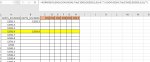
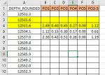
I have a very large spreadsheet that I am trying to return the value of some columns based on matching depths. Tab1 of my spreadsheet has no duplicate depths while Tab2 DOES have duplicate depths, some of which the columns have null values.

The attached Example Tab1 image has a yellow highlighted row that SHOULD contain data but, because the first value at this matching depth is null on the Example Tab 2 image, the result is blank. How do I get it to skip the null values and return the first non-null value? I have snagged my VLOOKUP statement in the image.

NOTE: Some columns will have text and others will be numbers. According to what I've read, I may need to use INDEX instead but I have yet been able to make heads or tails of the examples I've seen. Also, sorting is not an option as I have close to 500 columns to process.

Thank you for ANY help!
 

Attachments

  • Example Tab1.jpg
    Example Tab1.jpg
    86.5 KB · Views: 87
  • Example Tab2.jpg
    Example Tab2.jpg
    56.9 KB · Views: 87

Excel Facts

Create a chart in one keystroke
Select the data and press Alt+F1 to insert a default chart. You can change the default chart to any chart type
Have you tried using a pivot? Take the Depth Rounded Column as the Rows element and add the relevant columns to the Values area. That said, this might be tedious if you have over 500 columns (seems vast) to add to the values area. And what happens if a particular 'Depth Rounded' value has two or more lines with values in and one or more lines of blank or are there only ever no more than 2 lines (one blank and one with a value)?

Final thought, this may be much easier by creating your second table from the data table using Power Query - you can simply delete the rows with blanks.

Book.xlsx
ABCDEFGHIJKLMN
1Depth RoundedPO1Po2PO3PO4PO5Depth RoundedSum of PO1Sum of Po2Sum of PO3Sum of PO4Sum of PO5
212359.112359.1
312359.224681012359.2246810
412359.312359.312345
512359.31234512359.4678910
612359.467891012359.5
712359.512359.6
812359.612359.7
912359.712359.8
1012359.812359.9
1112359.912360
121236012360.1
1312360.112360.2
1412360.212360.3
1512360.3Grand Total913172125
Sheet3
 
Upvote 0
What version of Excel are you using?
If you have Excel 365 with the FILTER function then try this instead of the formula below.
IFERROR(FILTER(Sheet2!$B$2:$G$7,(Sheet2!$A$2:$A$7=Sheet1!$A2)*(Sheet2!$B$2:$B$7<>0)),"")
With the formula below copy the formula in C2 down and across.

Sheet1
Book1
ABCDEFGH
1Depth_RoundedDepth_RoundedPO1PO2PO3PO4PO5PO2-5
212531.312531.3      
312531.4      
412531.5      
512531.612531.62.490.40.450.2701.12
612531.7      
7125372.30.420.410.2601.19
812531.9      
Sheet1
Cell Formulas
RangeFormula
C2:H8C2=IFERROR(INDEX(Sheet2!$B$2:$G$6,AGGREGATE(15,6,(ROW(Sheet2!$A$2:$A$7)-ROW(Sheet2!$A$2)+1)/((Sheet2!$A$2:$A$7=Sheet1!$A2)*(Sheet2!$B$2:$B$7<>0)),1),MATCH(Sheet1!C$1,Sheet2!$B$1:$G$1,0)),"")


Sheet2
Book1
ABCDEFG
1Depth_RoundedPO1PO2PO3PO4PO5PO2-5
212531.3
312531.6
412531.62.490.400.450.270.001.12
512534.11.120.150.300.170.000.61
612537.02.30.420.410.260.001.19
712539.8
Sheet2
 
Upvote 0
If you have Excel 365 with the FILTER function then try this instead of the formula below.
IFERROR(FILTER(Sheet2!$B$2:$G$7,(Sheet2!$A$2:$A$7=Sheet1!$A2)*(Sheet2!$B$2:$B$7<>0)),"")
Hi AhoyNC
Just a couple of comments ..
  • Since this formula is on Sheet1 it doesn't need the Sheet1! reference. In fact it is a bad idea to include it. To see why, have a look at the example in post 11 here
  • You don't need the IFERROR with the FILTER function - at least not in this case if you have included it to deal with the situation where the FILTER function does not return any results. You can just use the optional 3rd argument of the FILTER function instead.

    =FILTER(Sheet2!$B$2:$G$7,(Sheet2!$A$2:$A$7=$A2)*(Sheet2!$B$2:$B$7<>0),"")
 
Upvote 0
Sorry - I see the duplication now. Your example show a whole row that is blank. How does it handle it if only some columns are blank?
 
Upvote 0
What version of Excel are you using?
If you have Excel 365 with the FILTER function then try this instead of the formula below.
IFERROR(FILTER(Sheet2!$B$2:$G$7,(Sheet2!$A$2:$A$7=Sheet1!$A2)*(Sheet2!$B$2:$B$7<>0)),"")
With the formula below copy the formula in C2 down and across.

Sheet1
Book1
ABCDEFGH
1Depth_RoundedDepth_RoundedPO1PO2PO3PO4PO5PO2-5
212531.312531.3      
312531.4      
412531.5      
512531.612531.62.490.40.450.2701.12
612531.7      
7125372.30.420.410.2601.19
812531.9      
Sheet1
Cell Formulas
RangeFormula
C2:H8C2=IFERROR(INDEX(Sheet2!$B$2:$G$6,AGGREGATE(15,6,(ROW(Sheet2!$A$2:$A$7)-ROW(Sheet2!$A$2)+1)/((Sheet2!$A$2:$A$7=Sheet1!$A2)*(Sheet2!$B$2:$B$7<>0)),1),MATCH(Sheet1!C$1,Sheet2!$B$1:$G$1,0)),"")


Sheet2
Book1
ABCDEFG
1Depth_RoundedPO1PO2PO3PO4PO5PO2-5
212531.3
312531.6
412531.62.490.400.450.270.001.12
512534.11.120.150.300.170.000.61
612537.02.30.420.410.260.001.19
712539.8
Sheet2
Darn....I'm running 2016
 
Upvote 0
If a column is blank the formula will return the values in the other columns. The blank column will return a 0 to Sheet1.
What do you want to happen?
 
Upvote 0
Sorry - I see the duplication now. Your example show a whole row that is blank. How does it handle it if only some columns are blank?

The default is that it will sum them together, though other behaviours are possible. That said, what do you want to happen?
 
Upvote 0
If some cells in a column can be blank then the formula I gave above will not work if a cell in column B is blank, but there is data in cells C - H in the same row.
One way around this would be to add a helper column on sheet B as in the example below. Also note the change of formula in cell C2.
IFERROR(INDEX(Sheet2!$B$2:$G$6,AGGREGATE(15,6,(ROW(Sheet2!$A$2:$A$7)-ROW(Sheet2!$A$2)+1)/((Sheet2!$A$2:$A$7=$A2)*(Sheet2!$I$2:$I$6)>0),1),MATCH(C$1,Sheet2!$B$1:$G$1,0)),"")

Sheet1
Book1
ABCDEFGH
1Depth_RoundedDepth_RoundedPO1PO2PO3PO4PO5PO2-5
212531.312531.3      
312531.4      
412531.5      
512531.612531.600.40.450.2701.12
612531.7      
7125372.30.4200.2601.19
812534.11.120.150.30.1700.61
Sheet1
Cell Formulas
RangeFormula
C2:H8C2=IFERROR(INDEX(Sheet2!$B$2:$G$6,AGGREGATE(15,6,(ROW(Sheet2!$A$2:$A$7)-ROW(Sheet2!$A$2)+1)/((Sheet2!$A$2:$A$7=$A2)*(Sheet2!$I$2:$I$6)>0),1),MATCH(C$1,Sheet2!$B$1:$G$1,0)),"")


Sheet2
Book1
ABCDEFGHI
1Depth_RoundedPO1PO2PO3PO4PO5PO2-5Sum
212531.30
312531.60
412531.60.40.450.2701.122.24
512534.11.120.150.30.1700.612.35
6125372.30.420.2601.194.17
712539.80
Sheet2
Cell Formulas
RangeFormula
I2:I7I2=SUM(B2:G2)
 
Upvote 0

Forum statistics

Threads
1,214,588
Messages
6,120,412
Members
448,959
Latest member
camelliaCase

We've detected that you are using an adblocker.

We have a great community of people providing Excel help here, but the hosting costs are enormous. You can help keep this site running by allowing ads on MrExcel.com.
Allow Ads at MrExcel

Which adblocker are you using?

Disable AdBlock

Follow these easy steps to disable AdBlock

1)Click on the icon in the browser’s toolbar.
2)Click on the icon in the browser’s toolbar.
2)Click on the "Pause on this site" option.
Go back

Disable AdBlock Plus

Follow these easy steps to disable AdBlock Plus

1)Click on the icon in the browser’s toolbar.
2)Click on the toggle to disable it for "mrexcel.com".
Go back

Disable uBlock Origin

Follow these easy steps to disable uBlock Origin

1)Click on the icon in the browser’s toolbar.
2)Click on the "Power" button.
3)Click on the "Refresh" button.
Go back

Disable uBlock

Follow these easy steps to disable uBlock

1)Click on the icon in the browser’s toolbar.
2)Click on the "Power" button.
3)Click on the "Refresh" button.
Go back
Back
Top