VLOOKUP (or INDEX/MATCH) with 2 criteria

[virtuosok]

Hi, appreciate your help...
I have a source tab (named mid3) in the following format (more rows and columns, too, some with blank entries):

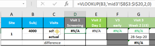
On a separate tab, in D3, I'm trying to set up a formula which would look up column B for matches with a reference cell and then return the value from adjacent cell in column C.

What am I doing wrong? I expected to have "23 Sep 2020" in this particular case. Also tried various solutions with INDEX/MATCH, changed formatting... =VLOOKUP(B3,'mid3'!$B$3:$I$20,2,0)

 

[Fluff]

The B3 cell the formula is using as the lookup value appears to be text, whereas the values on the mid3 sheet appear to be numbers.
Chagne B3 to a number & should be ok.

 

[virtuosok]

Thanks! No idea how I missed that!

 

[Fluff]

Glad to help & thanks for the feedback.