vlookup specific description from multiple tabs under specific header name in one column

[trpltwo]

Hi all, thank you advance for your help. Looking for a simple formula/vlookup to match some data across multiple tabs for reconciliation. Example attached.

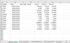
Master_Copy sheet = this is loaded into a system and sometimes the system have a habit of not being able to load all the prices in one go so it does it by batches.
“Price matched” tabs 1, 2 and 3 will show what is “matched_prices” and not matched which means what has been loaded successfully and not.
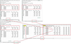
Ideally in tab sheet “Compare” from column I, I would like to have a formula/vlookup to look up from “Price matched 1” sheet to only capture any row under column header “Matched_Prices” only.
In each of the “Price matched” tabs 1, 2 and 3 sheet will have several columns headers and all consistence but I only want to look and capture rows under column header “Matched_Prices” only.

So in Compare sheet, I’m looking for code “AAA” therefore, look at “Price matched 1” tab and lookup under column header “Matched_Prices” if code “AAA” is there, if yes then copy or capture the row A to G, if not go to “Price matched 2” tab etc.

Hope I'm making sense. Thank you again in advance for your help.

 

[trpltwo]

I was trying to edit the title and the description but not sure how, apologies I'm still quite new.

Title should be vlookup specific description from multiple tabs under specific header name in one column.

I'm trying to do a VLOOKUP to look for a specific description/code that would be in multiple tabs however it has to be in specific header name/title that is located in a column that would have multiple headers.

To be more specific, from tab "Compare" cell I12 is "AAA" and I want to find the code "AAA" that is classified under header name "Matched_Prices" from column A across the multiple sheets "Price matched 1", "Price matched 2" and "Price matched 3" and grab data from column B to G.

So look for code "AAA" in sheets "Price matched 1" under column A with header name "Matched_Prices", if not there then look in next sheet name "Price matched 2" under column A with header name "Matched_Prices", if not there then look in next sheet name "Price matched 3". The sheet name "Price matched 3" will have "AAA" code so I want to be able to capture column B to G into the "compare" sheet from J12 - O12.
The purpose of this is to know which file the code is coming from and that all codes are accounted for under the "Matched_Prices".

Hope this is a little clearer.

 

[Peter_SSs]

I was trying to edit the title and the description but not sure how

You cannot edit the title but I have done that for you.
You can only edit your post for 10 minutes after posting. Otherwise just reply to the thread to clarify - as you have done.

 

[trpltwo]

You cannot edit the title but I have done that for you.
You can only edit your post for 10 minutes after posting. Otherwise just reply to the thread to clarify - as you have done.

Good to know thank you so much Peter_SSs

 

[fjns]

Hi, see the linked file for a possible solution...
Wrong cells visible on Google Drive, because Google Drive does not know the LET function. All formulas work correctly with your Office 365.

The formulas used in the table:
=LET(c,INDEX(Master_Copy!A:A,ROW()-1),IF(c="","",c))
=LET(i,IFERROR(MATCH(1,$Q3:$S3,-1),0),j,IFERROR(INDEX($Q3:$S3,i),0),d,IF(i=1,INDEX(Price_matched_1!B:B,j),IF(i=2,INDEX(Price_matched_2!B:B,j),IF(i=3,INDEX(Price_matched_3!B:B,j),""))),IF(d="","",d))
=LET(i,IFERROR(MATCH($I3,Price_matched_1!$A:$A,0),0),IF($A3="","",IF(AND(i>8,i<9+V$2),i,"")))

Compare.xlsx

 

[trpltwo]

Thank you so much for your response fjns. However, I was hoping for formulas to be populated from column J3 to O14 in the compare tab. So example
look for code "AAA" from compare sheet cell I12 in

1. sheets "Price matched 1" under column A with header name "Matched_Prices", if not there then
2. look in next sheet name "Price matched 2" under column A with header name "Matched_Prices", if not there then
3. look in next sheet name "Price matched 3". The sheet name "Price matched 3" will have "AAA" code so I want to be able to capture column B to G into the "compare" sheet from J12 - O12. ie "date", "Date", "Part Code", "Name", "Price 1", "Price 2", "Price 3" into Compare sheet from J12 to O12.

Hope this makes more sense.

 

[trpltwo]

Hi, see the linked file for a possible solution...
Wrong cells visible on Google Drive, because Google Drive does not know the LET function. All formulas work correctly with your Office 365.

The formulas used in the table:
=LET(c,INDEX(Master_Copy!A:A,ROW()-1),IF(c="","",c))
=LET(i,IFERROR(MATCH(1,$Q3:$S3,-1),0),j,IFERROR(INDEX($Q3:$S3,i),0),d,IF(i=1,INDEX(Price_matched_1!B:B,j),IF(i=2,INDEX(Price_matched_2!B:B,j),IF(i=3,INDEX(Price_matched_3!B:B,j),""))),IF(d="","",d))
=LET(i,IFERROR(MATCH($I3,Price_matched_1!$A:$A,0),0),IF($A3="","",IF(AND(i>8,i<9+V$2),i,"")))

Compare.xlsx

actually this is really good! realised this does help! thank you very much

 

[fjns]

Hi, I am very glad that the formulas work.
If I have enough knowledge, I am happy to help at any time.