VLOOKUP to extract multiple results - without vba

tinferns

Board Regular
Joined
Aug 18, 2009
Messages
150
Office Version
  1. 2019
  2. 2016
Platform
  1. Windows
Now, here's a tough one.... I am trying the below 2 formula's to obtain multiple results using index & Match formula. Doesn't seem to work. I am using Excel 2019 and Office 365. I want to avoid using VBA.

Formula's (options) used:
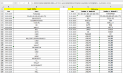
Index + Match1 = {=INDEX($B$3:$B$988,SMALL(IF(D3=$A$3:$A$988,ROW($A$3:$A$988)-ROW($A$3)+1),ROW(2:2)))}

Index + Match2 = {=INDEX($B$3:$B$987,SMALL(IF((D3=$A$3:$A$987),MATCH(ROW($A$3:$A$987),ROW($A$3:$A$987)),""),ROWS($C$2:C2)))}

Below is a screenshot of the above activity. Please help...

Thanks....
 

Attachments

  • Index n Match1.png
    Index n Match1.png
    69.3 KB · Views: 12

Excel Facts

What is the shortcut key for Format Selection?
Ctrl+1 (the number one) will open the Format dialog for whatever is selected.
Hi Peter SSs.. i tried adding or installing XL2BB add in.. not able to find it. This is too complex.. is there anyother way out so that I can share my document with you. ?
 

Attachments

  • xl2bb.png
    xl2bb.png
    47.4 KB · Views: 7
Upvote 0
Guess.. this is it..

Index n Match.xlsx
ABCDEF
1RAW DATAOutcome
2DateDataDateIndex + Match1Index + Match2
301-01-2020FORWARD01-01-202055+20+20+80+65+60+75)FORWARD
401-01-202055+20+20+80+65+60+75)01-01-2020#NUM!55+20+20+80+65+60+75)
502-01-20202819257677102-01-2020BDTECH-PG
602-01-2020Bank/MOPSDOAG02-01-2020WALLETBD
702-01-2020TECH-PG02-01-2020BILLWALLET
802-01-2020BD02-01-2020GUYSBILL
902-01-2020WALLET02-01-2020CARDGUYS
1002-01-2020BILL02-01-2020CARDCARD
1102-01-2020GUYS02-01-2020CCCARD
1202-01-2020CARD02-01-2020NAGARCC
1302-01-2020CARD02-01-2020#NUM!NAGAR
1403-01-2020 BIL/DEBIT/2020010301022303-01-2020#NUM!#NUM!
1503-01-2020CARD03-01-2020#NUM!#NUM!
1603-01-2020CARD03-01-2020#NUM!#NUM!
1703-01-2020WALLET03-01-2020#NUM!#NUM!
1804-01-20202822906727804-01-2020#NUM!#NUM!
1904-01-2020BELT04-01-2020#NUM!#NUM!
2004-01-2020CARD04-01-2020#NUM!#NUM!
2104-01-2020CC04-01-2020#NUM!#NUM!
2204-01-2020APPLE04-01-2020#NUM!#NUM!
2304-01-2020MICROSOFT04-01-2020#NUM!#NUM!
2404-01-2020CC04-01-2020#NUM!#NUM!
2504-01-2020WALLET04-01-2020#NUM!#NUM!
2605-01-2020KUMA/BHARATP05-01-2020#NUM!#NUM!
2705-01-2020CC05-01-2020#NUM!#NUM!
2805-01-2020CC05-01-2020#NUM!#NUM!
2905-01-2020MALL05-01-2020#NUM!#NUM!
3005-01-2020CC05-01-2020#NUM!#NUM!
3104-01-20202824034496604-01-2020#NUM!#NUM!
3207-01-20202827242079607-01-2020#NUM!#NUM!
3307-01-2020BOX.07-01-2020#NUM!#NUM!
3408-01-2020WALLET08-01-2020#NUM!#NUM!
3508-01-2020TWEET08-01-2020#NUM!#NUM!
3602-01-2020CC02-01-2020#NUM!#NUM!
3702-01-2020NAGAR02-01-2020#NUM!#NUM!
3809-01-2020E09-01-2020#NUM!#NUM!
3909-01-2020Rana09-01-2020#NUM!#NUM!
4009-01-20202830370768409-01-2020#NUM!#NUM!
4109-01-2020PG09-01-2020#NUM!#NUM!
4209-01-20202830381852009-01-2020#NUM!#NUM!
4310-01-20202833237120110-01-2020#NUM!#NUM!
4411-01-202011-01-2020#NUM!#NUM!
4511-01-2020267.5111-01-2020#NUM!#NUM!
4611-01-2020ONLY11-01-2020#NUM!#NUM!
4711-01-20202834751604111-01-2020#NUM!#NUM!
4811-01-20202834419025311-01-2020#NUM!#NUM!
4911-01-2020WALLET11-01-2020#NUM!#NUM!
5012-01-2020Mercha/BHARATP12-01-2020#NUM!#NUM!
5112-01-2020CARD12-01-2020#NUM!#NUM!
5212-01-2020Help12-01-2020#NUM!#NUM!
5312-01-20202835860506112-01-2020#NUM!#NUM!
5412-01-20202836341170712-01-2020#NUM!#NUM!
5513-01-20202836939473313-01-2020#NUM!#NUM!
5613-01-20202837784559613-01-2020#NUM!#NUM!
5714-01-2020zip/9900619235@okbi14-01-2020#NUM!#NUM!
5814-01-2020HOUS14-01-2020#NUM!#NUM!
5915-01-2020CC15-01-2020#NUM!#NUM!
6015-01-2020CARD15-01-2020#NUM!#NUM!
6115-01-2020WALLET15-01-2020#NUM!#NUM!
6217-01-2020BD17-01-2020#NUM!#NUM!
6317-01-202017-01-2020#NUM!#NUM!
6418-01-2020 PAYU-GROFERS-PG18-01-2020#NUM!#NUM!
6518-01-2020PG18-01-2020#NUM!#NUM!
6618-01-202018-01-2020#NUM!#NUM!
6718-01-2020CC18-01-2020#NUM!#NUM!
6818-01-2020ONLY18-01-2020#NUM!#NUM!
6918-01-20202845834857218-01-2020#NUM!#NUM!
7019-01-2020₹273.40 SUCCESS19-01-2020#NUM!#NUM!
7119-01-2020WALLET19-01-2020#NUM!#NUM!
7219-01-2020WALLET19-01-2020#NUM!#NUM!
7320-01-2020MUMBAI20-01-2020#NUM!#NUM!
7423-01-2020PG23-01-2020#NUM!#NUM!
7523-01-20202853680323723-01-2020#NUM!#NUM!
7623-01-2020SHOP23-01-2020#NUM!#NUM!
7725-01-2020CC25-01-2020#NUM!#NUM!
7825-01-20202856784303625-01-2020#NUM!#NUM!
7925-01-20202856781832825-01-2020#NUM!#NUM!
8025-01-2020WALLET25-01-2020#NUM!#NUM!
8126-01-20202857917206926-01-2020#NUM!#NUM!
8226-01-20202857777311626-01-2020#NUM!#NUM!
8326-01-202026-01-2020#NUM!#NUM!
8426-01-2020WALLET26-01-2020#NUM!#NUM!
8529-01-2020BIRTHDAY29-01-2020#NUM!#NUM!
8631-01-2020Jan31-01-2020#NUM!#NUM!
8721-01-2020PL-INDIA21-01-2020#NUM!#NUM!
8801-02-20202866658506101-02-2020#NUM!#NUM!
8901-02-20202867164885401-02-2020#NUM!#NUM!
9001-02-2020CARD01-02-2020#NUM!#NUM!
9101-02-2020ACCOUNT- UPI/003215200697/Med/rameshbillava01/Can01-02-2020#NUM!#NUM!
9201-02-20202867211196201-02-2020#NUM!#NUM!
9301-02-2020537/0146801-02-2020#NUM!#NUM!
9401-02-2020NAGAR01-02-2020#NUM!#NUM!
9501-02-20202867429756401-02-2020#NUM!#NUM!
9601-02-20202867463411101-02-2020#NUM!#NUM!
9701-02-2020Mercha/BHARATP01-02-2020#NUM!#NUM!
9802-02-20202868149471602-02-2020#NUM!#NUM!
9902-02-2020ID 407-9334553-637076302-02-2020#NUM!#NUM!
10002-02-2020ID 407-9964547-461392002-02-2020#NUM!#NUM!
Sheet1
Cell Formulas
RangeFormula
E3:E100E3=INDEX($B$3:$B$988,SMALL(IF(D3=$A$3:$A$988,ROW($A$3:$A$988)-ROW($A$3)+1),ROW(2:2)))
F3:F100F3=INDEX($B$3:$B$987,SMALL(IF((D3=$A$3:$A$987),MATCH(ROW($A$3:$A$987),ROW($A$3:$A$987)),""),ROWS($C$2:C2)))
Press CTRL+SHIFT+ENTER to enter array formulas.
Cells with Conditional Formatting
CellConditionCell FormatStop If True
D3:D987Expression="t6>=1000"textNO
A3:A1326Expression="t6>=1000"textNO
 
Upvote 0
Guess.. this is it..
Indeed it is. (y)
The only thing is I would like to see the results that you do want (with explanation) in columns D:F, not the results you don't want. ;)
 
Upvote 0
Thanks Peter SSs. My expectations are as below:

1) I want all the results from column B to show up in Column D or F. One challenge is that you may find 01/01/20 between row 5 - 10 and randomly in say row 250 !. So here I want all 11 outputs.
2) Lets use the same example. The date 01/01/20 appears only 11 times. However, in column D I put that date 12 times, I want the output to be either 0 or - for the 12th entry.

Guess, this is do'able. Please let me know if you need more information. Thanks..
 
Upvote 0
I don't understand your written description of your requirements. Can you show the expected results(or at least several of them) for the sample data given and explain in relation to those examples?
 
Upvote 0
Sure Peter SSs. Below example I have done manually.

What you will observe:
1) In outcome section, dates are not placed in a proper sequence. I have highlighted in orange to show the mix. I am not concerned about hierarchy and sequence of data in output. As long its all there.
2) In Raw Data there are only 3 entries for 01/01/20. However in Outcome, we are seeking information for 4 entries of 01/01/20 - thus the 4th entry gets a 0
3) In raw data there are 6 entries for 04/01/20. However in outcome we are seeking only 4 entries. Thus Bangkok & Pattaya is missed out in outcome. Which is fine.

The above 2 formula's are fine, however in some cases I am getting errors. I hope the above explanations should do. Please advise if you want me to deeper.

Thanks,

Index n Match.xlsx
ABCDE
1RAW DATAOutcome
2DateDataDateIndex + Match1
301-01-2020Boston01-01-2020Boston
401-01-2020New Orleans01-01-2020New Orleans
502-01-2020Paris02-01-2020Paris
602-01-2020Frankfurt02-01-2020Frankfurt
702-01-2020Amsterdam02-01-2020Amsterdam
802-01-2020Prague02-01-2020Prague
902-01-2020London02-01-2020London
1002-01-2020Athens02-01-2020Athens
1102-01-2020Geneva02-01-2020Geneva
1202-01-2020Manchester02-01-2020Manchester
1302-01-2020Brussels03-01-2020Melbourne
1403-01-2020Melbourne03-01-2020Sydney
1503-01-2020Sydney03-01-2020Cairns
1603-01-2020Cairns04-01-2020Singapore
1703-01-2020Queensland04-01-2020Hongkong
1804-01-2020Singapore01-01-2020Chicago
1904-01-2020Hongkong04-01-2020Bejeing
2004-01-2020Bangkok04-01-2020Bali
2104-01-2020Bejeing01-01-20200
2204-01-2020Bali02-01-2020Brussels
2304-01-2020Pattaya02-01-2020Cairo
2401-01-2020Chicago02-01-2020Moscow
2502-01-2020Cairo03-01-2020Queensland
2602-01-2020Moscow03-01-20200
Sheet2
Cells with Conditional Formatting
CellConditionCell FormatStop If True
A3:A26,D3:D26Expression="t6>=1000"textNO
 
Upvote 0
How about
+Fluff v2.xlsm
ABCDE
1RAW DATAOutcome
2DateDataDateIndex + Match1
301/01/2020Boston01/01/2020Boston
401/01/2020New Orleans01/01/2020New Orleans
502/01/2020Paris02/01/2020Paris
602/01/2020Frankfurt02/01/2020Frankfurt
702/01/2020Amsterdam02/01/2020Amsterdam
802/01/2020Prague02/01/2020Prague
902/01/2020London02/01/2020London
1002/01/2020Athens02/01/2020Athens
1102/01/2020Geneva02/01/2020Geneva
1202/01/2020Manchester02/01/2020Manchester
1302/01/2020Brussels03/01/2020Melbourne
1403/01/2020Melbourne03/01/2020Sydney
1503/01/2020Sydney03/01/2020Cairns
1603/01/2020Cairns04/01/2020Singapore
1703/01/2020Queensland04/01/2020Hongkong
1804/01/2020Singapore01/01/2020Chicago
1904/01/2020Hongkong04/01/2020Bangkok
2004/01/2020Bangkok04/01/2020Bejeing
2104/01/2020Bejeing01/01/2020-
2204/01/2020Bali02/01/2020Brussels
2304/01/2020Pattaya02/01/2020Cairo
2401/01/2020Chicago02/01/2020Moscow
2502/01/2020Cairo03/01/2020Queensland
2602/01/2020Moscow03/01/2020-
Main
Cell Formulas
RangeFormula
E3:E26E3=IFERROR(INDEX($B$3:$B$26,AGGREGATE(15,6,(ROW($B$3:$B$26)-ROW($B$3)+1)/($A$3:$A$26=D3),COUNTIF(D$3:D3,D3))),"-")
 
Upvote 0
Solution
Thanks Fluff.. That Formula did the trick.. and did it well. Thanks a ton..
 
Upvote 0

Forum statistics

Threads
1,214,593
Messages
6,120,435
Members
448,962
Latest member
Fenes

We've detected that you are using an adblocker.

We have a great community of people providing Excel help here, but the hosting costs are enormous. You can help keep this site running by allowing ads on MrExcel.com.
Allow Ads at MrExcel

Which adblocker are you using?

Disable AdBlock

Follow these easy steps to disable AdBlock

1)Click on the icon in the browser’s toolbar.
2)Click on the icon in the browser’s toolbar.
2)Click on the "Pause on this site" option.
Go back

Disable AdBlock Plus

Follow these easy steps to disable AdBlock Plus

1)Click on the icon in the browser’s toolbar.
2)Click on the toggle to disable it for "mrexcel.com".
Go back

Disable uBlock Origin

Follow these easy steps to disable uBlock Origin

1)Click on the icon in the browser’s toolbar.
2)Click on the "Power" button.
3)Click on the "Refresh" button.
Go back

Disable uBlock

Follow these easy steps to disable uBlock

1)Click on the icon in the browser’s toolbar.
2)Click on the "Power" button.
3)Click on the "Refresh" button.
Go back
Back
Top