Vlookup Variable offset

[Onearmedscizor]

Windows 7, Office 2010

Sample Data

Sku	Description	Ordered	MODE
1234	Widget 1
		4
		6
		6
		6	6

<tbody>
</tbody>

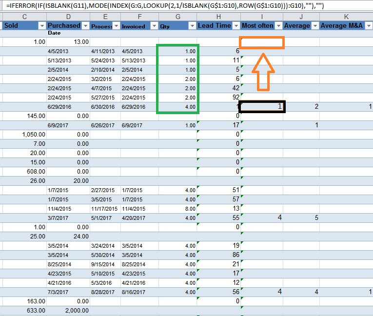
Mode, column 4, has the following formula:
=IFERROR(IF(ISBLANK(C6),MODE(INDEX(C:C,LOOKUP(2,1/ISBLANK(C$1:C5),ROW(C$1:C5))):C5),""),"")

The only issue with this is that the result is inserted at the end of the list. Or right before the next black cell. I am going to utilize the result in column 4 in a Vlookup formula with the SKU number. The issue is the vlookup result will be blank because the result in column 4 is offset.

My question is: is there a way I can modify the formula above to have a result inserted into D1? Or what is the best way to utilize the results of the formula.

Let me know if i need to explain this better.

 

[Scott T]

Is this what you want?

[RANGE=cls:xl2bb-100][XR][XH=cs:5]Excel 2010[/XH][/XR][XR][XH][/XH][XH]A[/XH][XH]B[/XH][XH]C[/XH][XH]D[/XH][/XR][XR][XH]1[/XH][XD=h:l]Sku[/XD][XD=h:l]Description[/XD][XD=h:l]Ordered[/XD][XD=h:l]MODE[/XD][/XR][XR][XH]2[/XH][XD=h:r]1234[/XD][XD=h:l]Widget 1[/XD][XD=h:r][/XD][XD=h:r|cls:fx][FORMULA==MODE(C3:INDEX(C:C,MATCH(99999,C:C)))]6[/FORMULA][/XD][/XR][XR][XH]3[/XH][XD=h:r][/XD][XD=h:r][/XD][XD=h:r]4[/XD][XD=h:r][/XD][/XR][XR][XH]4[/XH][XD=h:r][/XD][XD=h:r][/XD][XD=h:r]6[/XD][XD=h:r][/XD][/XR][XR][XH]5[/XH][XD=h:r][/XD][XD=h:r][/XD][XD=h:r]6[/XD][XD=h:r][/XD][/XR][XR][XH]6[/XH][XD=h:r][/XD][XD=h:r][/XD][XD=h:r]6[/XD][XD=h:r][/XD][/XR][XR][XH]7[/XH][XD=h:r][/XD][XD=h:r][/XD][XD=h:r][/XD][XD=h:r][/XD][/XR][XR][XH=cs:5][RANGE][XR][XD]Sheet6[/XD][XH][/XH][/XR][/RANGE][/XH][/XR][/RANGE][RANGE=cls:xl2bb-extra-100][XR][XH=cs:2|h:l|fw:b]Cell Formulas[/XH][/XR][XR][XH]Cell[/XH][XH]Formula[/XH][/XR][XR][XD]D2[/XD][XD]=MODE(C3:INDEX(C:C,MATCH(99999,C:C)))[/XD][/XR][/RANGE]

 

[Onearmedscizor]

It is what i am looking for but i have 51,580 rows. So i don't know how to incorporate your code into my existing formula:

=IFERROR(IF(ISBLANK(G11),MODE(INDEX(G:G,LOOKUP(2,1/ISBLANK(G$1:G10),ROW(G$1:G10))):G10),""),"")

What i am doing is finding the numbers most often occurring between two blank cells. So that formula inserts the result right before the next blank cell. I don't know how to have it inserted into the first blank cell adjacent to the column it is computing "MODE" on.

I have taken a screenshot of what needs to be done. Basically like your formula, but using the formula i already have:

Outlined in green is the what is being computed. Black is where the data is currently being inserted, orange is where i would like it to be (because i need to use it in a vlookup, referencing the SKU which inst pictured).