Vlookup with indirect returning 0, when value is present

[ChrisTag1]

Hey everyone,

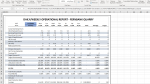
Looking for some help again. I have a formula..... =IFERROR(IF($G$8="Primary",VLOOKUP(I$8,INDIRECT("PrimaryDailyRange"),2,0),IF($G$8="Secondary",VLOOKUP(I$8,INDIRECT("SecondaryDailyRange"),2,0))),0),
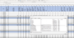
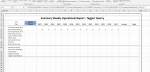
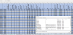
that works exactly how I need it to in one worksheet. The next worksheet is almost exactly the same as the first, except I am getting the data from a different named range. I am trying to use this same formula with the new named range, but it returns 0 instead of the data in the referenced cell. =IFERROR(IF($G$8="Primary",VLOOKUP(U$8,INDIRECT("PrimaryWeeklyRange"),2,0),IF($G$8="Secondary",VLOOKUP(U$8,INDIRECT("SecondaryWeeklyRange"),2,0))),0)
What am I doing wrong? I don't understand why it works for one named range and not for the other.

Any ideas?

Thanks all.

 

[mole999]

Don't know but your primaryweekly range seems to have a space as the first part of the data, in which case it maybe the IFEEROR is triggered which is why the zero. If you made 0 into a word you would see its the error trap

 

[FatBoyClam]

Looks to me like the 0 it's returning is likely to be the result of the IFERROR function.

Try taking the IFERROR out, or using the inline evaluation of the formula to check for errors.
My guess would be that the date you're looking up doesn't actually exist in the lookup table (the years are not displayed, so can't be certain one way or the other)

 

[FatBoyClam]

Also - as far as I see the use of Indirect here is redundant (you can just use the range name directly in the vlookup formula).

However, you could simplify your formula (and make it more efficient) by leveraging the naming convention and the INDIRECT function;

=IFERROR(VLOOKUP(U$8,INDIRECT($G$8&"WeeklyRange"),2,0),0)

This concatenates the value from G8 (Primary or Secondary) with "WeeklyRange" (common between the two range names), and feeds it into the INDIRECT function to get a reference to the relevant range.

This should be a more efficient option, where your formula is doing two cell comparisons (the test part of the IF statements) and two VLOOKUPS (Excel evaluates every element of a formula), where the above does one INDIRECT and one VLOOKUP.

 

[ChrisTag1]

FatBoyClam,
I redid the formula without the IFERROR, and the error I am getting is #NA. I thought it was the dates too, but the dates are all the same in every worksheet. So in the first worksheet, where the formula works, it is looking up the same dates as in the second worksheet. So I am really at a loss as to why I can't get my formula to return a value that I can plainly see is in the cell.

 

[ChrisTag1]

FatBoyClam,
You were correct about the date. In the 2 tables being referenced in my formula, the date was a text instead of a date. (ie "10/28/19" instead of 43766). I have been so used to the answers to my problems being complicated that I completely overlooked the obvious.

Cheers

 

[FatBoyClam]

Glad you got to the answer Chris
Hope the shortened formula works for you, if you try it out.