Vlookup with multiple conditions

[olivera87]

Hello,

I ask for your help. I would like to optimize my everyday work, since now it is devided into many excel files that take long to check them all. I have joined all the excel files into one, and now I need help to set up an automatic output cell that would agree with many conditions.

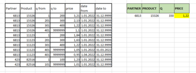
So we have columns: CUSTOMER CODE (3-5 numbers usually), PRODUCT CODE (also 3-5 numbers usually), QUANTITY, PRICE, DATE. There are many customers that have some of the same products, with a price (unique for every partner) that depends on the order quantity (the more products you order, the lower the price). Example: customer 12546 has a product 5555 for a price 2,10 eur if they order 100 pcs, 2,00 eur for 200 pcs, and 1,6 eur for 500 pcs). The quantity is unique for every partner, just like the prices. The date is important since the price can change in the future and I would like to only enter a new period and price when it does.

My wish is to have a sheet with a table where I would write: CUSTOMER CODE, PRODUCT CODE, QUANTITY AND DATE manualy and the PRICE per pcs would be shown automaticly in the next cell considering the conditions. I attached the picture of how the data base would look, and what I would like to get out with a formula.

Please help me, which function would be the best. As I researched, VLOOK would not be the best for this.

Thank you so much for your help.

 

[kweaver]

Welcome to Mr. Excel,

It would help greatly if you show your sample using XL2BB so that retyping your data isn't required on the part of someone helping you.

Using 365, does this do it in M3?

=FILTER(F3:F13,(J3=B3:B13)*(K3=C3:C13)*(L3>=D3:D13)*(L3<=E3:E13))

Book5
	B	C	D	E	F	G	H	I	J	K	L	M
2	Partner	product	from	to	price				Partner	Product	Q	Price
3	6813	15326	1	200	3.21				6813	15326	350	1.22
4	6813	15326	201	300	2.13
5	6813	15326	301	400	1.22
6	6813	15326	401	9999999	1.1
7	6813	11123	1	200	1.84
8	6813	11123	201	300	1.63
9	6813	11123	301	400	1.22
10	6813	11123	401	9999999	1.05
11	6813	11123	401	9999999	0.95
12	423	82516	1	100	1.23
13	423	82516	101	9999999	1.01
Sheet1

Cell Formulas
Range	Formula
M3	M3	=FILTER(F3:F13,(J3=B3:B13)*(K3=C3:C13)*(L3>=D3:D13)*(L3<=E3:E13))

 

[Peter_SSs]

Welcome to the MrExcel board!

My wish is to have a sheet with a table where I would write: CUSTOMER CODE, PRODUCT CODE, QUANTITY AND DATE manualy and the PRICE per pcs would be shown automaticly in the next cell considering the conditions. I attached the picture of how the data base would look, and what I would like to get out with a formula.

Seems like Date is missing from your results section. If that is to be included then you would need to add a further two bracketed sections to the formula suggested above to account for the date.
Alternatively, if you want the formula to work in all your Excel versions, you could try this. It assumes that only a single row of the original data would meet all the conditions given.

22 05 22.xlsm
	A	B	C	D	E	F	G	H	I	J	K	L	M	N
1
2		Partner	Product	q from	q to	price	date from	date to		PARTNER	PRODUCT	Q	DATE	PRICE
3		6813	15326	1	200	3.21	1/01/2022	31/12/9999		6813	15326	350	21/01/2022	1.22
4		6813	15326	201	300	2.13	1/01/2022	31/12/9999		6813	11123	410	23/04/2022	0.95
5		6813	15326	301	400	1.22	1/01/2022	31/12/9999		423	82516	100	2/02/2022	1.23
6		6813	15326	401	9999999	1.1	1/01/2022	31/12/9999
7		6813	11123	1	200	1.84	1/01/2022	31/12/9999
8		6813	11123	201	300	1.63	1/01/2022	31/12/9999
9		6813	11123	301	400	1.22	1/01/2022	31/12/9999
10		6813	11123	401	9999999	1.05	1/01/2022	31/03/2022
11		6813	11123	401	9999999	0.95	1/04/2022	31/12/9999
12		423	82516	1	100	1.23	1/01/2022	31/12/9999
13		423	82516	101	9999999	1.01	1/01/2022	31/12/9999
14
Lookup Price

Cell Formulas
Range	Formula
N3:N5	N3	=SUMIFS(F$3:F$13,B$3:B$13,J3,C$3:C$13,K3,D$3:D$13,"<="&L3,E$3:E$13,">="&L3,G$3:G$13,"<="&M3,H$3:H$13,">="&M3)

 

[olivera87]

Thank you all for your help. I entered this formulas and I did not show me the result, it wrote an error. I copied it into the cell and it didn't work. Was I supposed to change something? Sorry if I am asking very basic questions, but I am new to this.

I put a little more thinking into it and it would be great if the part where you put un inquery like partner, article, q and date would be in a seperate sheet (worksheet 2 in same file), so I could use it to import in our program.

Is this possible?

Thank you.

 

[olivera87]

Update, the formula =SUMIFS(F$3:F$13,B$3:B$13,J3,C$3:C$13,K3,D$3:D$13,"<="&L3,E$3:E$13,">="&L3,G$3:G$13,"<="&M3,H$3:H$13,">="&M3) works great! Thank you so much

Now my only wish is, that it could be moved to another sheet. Any ideas?

 

[kweaver]

Can't you just change the references based on the other sheet?

Something like:

=SUMIFS(Sheet1!F$3:F$13,Sheet1!$B$3:$B$13,B3,Sheet1!C$3:C$13,C3,Sheet1!D$3:D$13,"<="&D3,Sheet1!E$3:E$13,">="&D3,Sheet1!G$3:G$13,"<="&E3,Sheet1!H$3:H$13,">="&E3)

With this formula in F3 and filled down and the data in B3:F5

 

[olivera87]

Can't you just change the references based on the other sheet?

Something like:

=SUMIFS(Sheet1!F$3:F$13,Sheet1!$B$3:$B$13,B3,Sheet1!C$3:C$13,C3,Sheet1!D$3:D$13,"<="&D3,Sheet1!E$3:E$13,">="&D3,Sheet1!G$3:G$13,"<="&E3,Sheet1!H$3:H$13,">="&E3)

With this formula in F3 and filled down and the data in B3:F5

Thank you so much, works perfectly!

 

[kweaver]

Glad to help.

 

[olivera87]

Welcome to Mr. Excel,

It would help greatly if you show your sample using XL2BB so that retyping your data isn't required on the part of someone helping you.

Using 365, does this do it in M3?

=FILTER(F3:F13,(J3=B3:B13)*(K3=C3:C13)*(L3>=D3:D13)*(L3<=E3:E13))

Book5
	B	C	D	E	F	G	H	I	J	K	L	M
2	Partner	product	from	to	price				Partner	Product	Q	Price
3	6813	15326	1	200	3.21				6813	15326	350	1.22
4	6813	15326	201	300	2.13
5	6813	15326	301	400	1.22
6	6813	15326	401	9999999	1.1
7	6813	11123	1	200	1.84
8	6813	11123	201	300	1.63
9	6813	11123	301	400	1.22
10	6813	11123	401	9999999	1.05
11	6813	11123	401	9999999	0.95
12	423	82516	1	100	1.23
13	423	82516	101	9999999	1.01
Sheet1

Cell Formulas
Range	Formula
M3	M3	=FILTER(F3:F13,(J3=B3:B13)*(K3=C3:C13)*(L3>=D3:D13)*(L3<=E3:E13))

Hello,

can you please help me add a condition of date into the code.
Thank you.

 

[olivera87]

Glad to help.

Update, it works great but there is a problem, that when you enter a product with two different prices to mach both conditions, it sums them together.

To explain in example: partner 423, product 4152, q 100-200, price 1,50 and another entry: partner 423, product 4152, q 200-1000 price 1,52 the result will be price 3,02 for q (for example) 200.

Is it possible to use a different code, that would like select a smaller price in this case?

I fully understand the base file (all the data) has to be cleared and that the duplicat values are not allowed, but at the volume of product we have in our base it can happen quickly.

I hope you understand what I wrote.

Thank you.