Vlookup with Multiple Criteria

[Joraemonn]

Hi all,
I need help with one of my formulas.
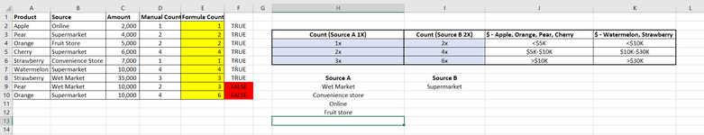
- The table in col. H to K row 3 to 6 shows the criteria (product, source, amount). Col. H Row 8 to to 12 is Source A, Col I Row 8 to 9 is Source B. The one in blue is the result that i want based on the criteria.
E.g. If product = Apple, Source = Online (Source A), Amount = $2000 -> it should give me the result of 1 count.

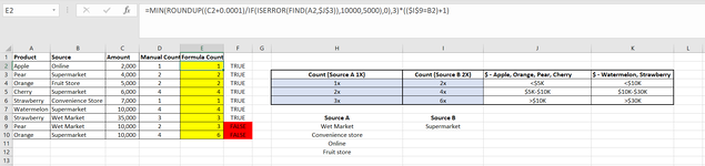
I input the formula but I can't get the right answer for row 9 and 10. The formula I'm using is: =MIN(ROUNDUP((C2+0.0001)/IF(ISERROR(FIND(A2,$J$3)),10000,5000),0),3)*(($I$9=B2)+1)
Not sure what is missing from my formula. Appreciate if anyone can help with that.
Thank you.

 

[jasonb75]

I've got a bit of a theory that I'm working on but I could be way off of what you actually want. In all honesty, I think that you will need to explain how you calculated your manual results rather than assuming that people will automatically understand what you're trying to do.

 

[jasonb75]

After cleaning up your reference table and throwing the original formula away I've been able to work out what you're trying to do along with a couple of working alternatives. In my opinion it was more the wrong approach to the task than something missing from the formula.

Book1
	A	B	C	D	E	F	G	H	I	J	K
1					Formula	Alt formula
2	Apple	Online	2000	1	1	1
3	Pear	Supermarket	4000	2	2	2		Wet Market,Convenience Store,Online,Fruit Store	Supermarket	Apple, Orange, Pear, Cherry	Watermelon, Strawberry
4	Orange	Fruit Store	5000	2	2	2		1	2	0	0
5	Cherry	Supermarket	6000	4	4	4		2	4	5000	10000
6	Strawberry	Convenience Store	7000	1	1	1		3	6	10000.01	30000.01
7	Watermelon	Supermarket	10000	4	4	4
8	Strawberry	Wet Market	35000	3	3	3
9	Pear	Wet Market	10000	2	2	2
10	Orange	Supermarket	10000	4	4	4
Sheet3

Cell Formulas
Range	Formula
E2:E10	E2	=LOOKUP(C2,XLOOKUP("*"&A2&"*",$J$3:$K$3,$J$4:$K$6,,2),XLOOKUP("*"&B2&"*",$H$3:$I$3,$H$4:$I$6,,2))
F2:F10	F2	=INDEX($H$4:$I$6,MATCH(C2,INDEX($J$4:$K$6,,MATCH(2,1/ISNUMBER(SEARCH(A2,$J$3:$K$3))))),MATCH(2,1/ISNUMBER(SEARCH(B2,$H$3:$I$3))))

 

[Joraemonn]

Hi Jason75,
Sorry for not being specific to what I need and I think your answer may be slightly way off of what I need.
- 2 sources - Source A and Source B. Wet Market / Convenience store / Online / Fruit Store are categorized as Source A. Supermarket categorized as Source B.
- 2 groups of products: Apple / Orange / Pear / Cherry in 1 group (let's name it as Group 1 - cell:J3) . Watermelon / Strawberry in 2nd group (Group 2 - cell:K3)
- For amount in Group 1, it is categorized into 3: <$5000 (J4) / $5000 to $10000 (J5) / >$10000 (J6). For amount in Group 2, it is categorized: <$10000 (K4) / $10000 to $30000 (K5) / >$30000 (K6)
- What i need is if i have a product, source and amount, it should pick up the number in H4:I6 (in blue).
- Example in row 2: Product = Apple (J3 - refer to only col. J for apple), Source = Online (Online falls under Source A which H3 - refer to only col. H for source A), Amount = $2000 (which is <$5000 - refer to J4), hence answer should be 1 (H4)
- Example in row 4: Product = Pear (J3 - refer to only col. J for pear), Source = Supermarket (Supermarket falls under Source B which I3 - refer to only col. I for source B), Amount = $4000 (which is <$5000 - refer to J4), hence answer should be 2 (I4)
- Example in row 9: Product = Pear (J3 - refer to only col. J for pear), Source = Wet Market (Wet Market falls under Source A which H3 - refer to only col. H for source A), Amount = $10000 (which falls under $5000 to $10000 - refer to J5), hence answer should be 2 (H5)

I hope with the explanation above, you might have a better picture of what I need. Hope you are able to help. Thank you.

 

[jasonb75]

Hi, reading your description above, I can't see any difference between that and what I have done. I've just taken a different approach in order to try and be more consistent and formula friendly.

The bit that might not make sense at a glance (sorry, I should have explained the logic in my earlier reply) is the way that I've changed columns J and K.

Looking specifically at column J, there are 3 values,
0
5000
10000.01

Comparing those to what you originally had in the same cells, they are the lowest permissible values for <$5000, $5000-$10000, and >$10000 respectively. A formula can not read 2 numbers in the same cell as a range so the best way is to set the lowest value in each of the ranges then use an approximate match to find the highest value that is less than or equal to the criteria.

The 2 methods that I used both work on the principle of taking the content of column A and searching for it in J3 and K3.
They then search for the highest value in the 3 numbers below J3 or K3 (whichever one matched to column A) that is less than or equal to the value in column C.
Finally they search for the content of column C in H3 and I3, then return the value from the cell where this match and the row where the value in the previous step intersect.

Hopefully that makes a bit of sense, I can understand it a lot easier than I can explain it.

One thing to point out (assuming that the sample data is fictional) there will be a risk of incorrect partial matches for similar strings.
For example, if you had Pineapple in K3 then apple would be matched to it in error. There are ways to prevent this if needed but I won't add them in until the rest of it is correct.