sjohnson77
New Member
- Joined
- Apr 17, 2021
- Messages
- 11
- Office Version
- 365
- 2019
- Platform
- Windows
Hi Guys ")
I am a novice Excel user who is looking to automate my workload to save me time.
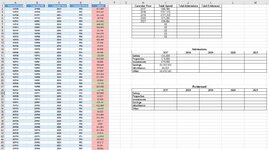
I am currently working on a financial project for my business and I have attached a screenshot to show what I am talking about.
I have my data which gets pulled automatically on the left and then I have my analysis tables ready on the right. So far I have automated the total spend column to calculate the total spend correctly depending on the year selected in the drop down (top table).
I now am working on a way to total the amounts in the admissions & Evidenced tables (Salary, properties investments etc.) and to collectively total the admissions/Evidence automatically in the top table corresponding to the correct year. Is there a formula I can use to automate this for me? I will be manually typing the admissions and evidenced values in anyway (middle table and bottom table on the right), but I want a way for the spreadsheet to calculate all the values collectively and to show the values in the table at the top once I have typed them in?
Any help would be greatly appreciated!
Kind regards
I am a novice Excel user who is looking to automate my workload to save me time.
I am currently working on a financial project for my business and I have attached a screenshot to show what I am talking about.
I have my data which gets pulled automatically on the left and then I have my analysis tables ready on the right. So far I have automated the total spend column to calculate the total spend correctly depending on the year selected in the drop down (top table).
I now am working on a way to total the amounts in the admissions & Evidenced tables (Salary, properties investments etc.) and to collectively total the admissions/Evidence automatically in the top table corresponding to the correct year. Is there a formula I can use to automate this for me? I will be manually typing the admissions and evidenced values in anyway (middle table and bottom table on the right), but I want a way for the spreadsheet to calculate all the values collectively and to show the values in the table at the top once I have typed them in?
Any help would be greatly appreciated!
Kind regards