Workbook Comparison - Weekly Entry Delta

[Gsrgofass]

Hello All,

I have a Master list of data. Each week, I get an updated list where some items can drop off OR new items could be added OR both.
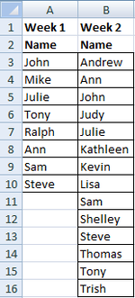
Good news is I only need to be concerned with the delta of the ‘Name’ column in order to determine the weekly changes, if any.

Each week I would like to compare the old list with the new list and have some clear visibility of the items that have been added and the items that could have potentially dropped off the list.

If this week’s list had 20 items and next week 10 new names are added and 5 names dropped off, a list of all 35 names. The resulting list, after next week’s list, would show the names that have remained unchanged, the names that have dropped off and the new names added. The reason I need to know which names dropped off or new ones that were added is because I have to report on these changes. Maybe color the cells that dropped off in RED and new names in YELLOW leaving unchanged names uncolored?

I am unsure whether I can do this with VLOOKUP with some additional functions and conditional formatting or if I should be doing this with Power Query. This is why I’m posting here first. If Power BI is the solution, I can post this question there.

Thanks all. Hope everyone has a great wknd.

Steve

 

[AhoyNC]

Maybe something like this:

Book1
	A	B	C	D	E
1	Week 1	Week 2		Added	Removed
2	Name	Name		Names	Names
3	John	Andrew		Andrew	Mike
4	Mike	Ann		Judy	Ralph
5	Julie	John		Kathleen
6	Tony	Judy		Kevin
7	Ralph	Julie		Lisa
8	Ann	Kathleen		Shelley
9	Sam	Kevin		Thomas
10	Steve	Lisa		Trish
11		Sam
12		Shelley
13		Steve
14		Thomas
15		Tony
16		Trish
Sheet2

Cell Formulas
Range	Formula
E3:E8	E3	=IFERROR(INDEX($A$3:$A$106,AGGREGATE(15,6,(ROW($B$3:$B$16)-ROW($B$3)+1)/(ISNA(MATCH($A$3:$A$10,$B$3:$B$16,0))),ROWS($D$3:D3))),"")
D3:D13	D3	=IFERROR(INDEX($B$3:$B$16,AGGREGATE(15,6,(ROW($B$3:$B$16)-ROW($B$3)+1)/(ISNA(MATCH($B$3:$B$16,$A$3:$A$10,0))),ROWS($D$3:D3))),"")

Cells with Conditional Formatting
Cell	Condition		Cell Format	Stop If True
B3:B16	Expression	=ISNA(MATCH(B3,$A$3:$A$10,0))	text	NO
A3:A10	Expression	=ISNA(MATCH(A3,$B$3:$B$16,0))	text	NO

 

[Gsrgofass]

This works great, thanks!!!!

Would you mind breaking this formula and cond. formatting down so I can understand how it works, please?
With me understanding it more clearly I can hopefully expand my knowledge of Excel.

 

[AhoyNC]

This link will explain the formula. I used the IFERROR function instead of the count function which is used in the video. He is right that the IFERROR function can slow down a worksheet if it has a lot of formulas. In most cases you probably won't notice a difference.

 

[Gsrgofass]

This link will explain the formula. I used the IFERROR function instead of the count function which is used in the video. He is right that the IFERROR function can slow down a worksheet if it has a lot of formulas. In most cases you probably won't notice a difference.

Right on for the formula. Any help the cond formatting?

 

[AhoyNC]

On ribbon go to Conditional Formatting
- New Rule
- Use a formula .......
Then to format removed names but in this formula =ISNA(MATCH(A3,$B$3:$B$16)
change above formula to match your data.

For added names