Working out RAG status based on 3 columns

[theguyIsHere]

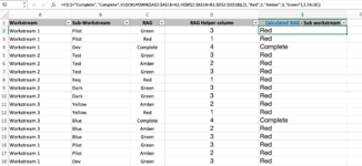
Trying to summarise the RAG status in one field but unsure how I do that

Column D needs to make sure it groups Column A and then column B and then assign the lowest RAG from column C

For example, For Workstream 1, 'Pilot' appears twice in column B with the lowest RAG status of Red. So Column D automatically needs to assign Red to Workstream 1, pilot sub workstream.

If it is easier then RAG status could be assigned a number too. For example: Red = 1, Amber = 2, Green = 3, Complete = 4 etc

Table with dummy data below. Grateful for any assistance on this, please.

Column A	Column B	Column C	Column D
Workstream	Sub-Workstream	RAG	Calculated RAG - Sub workstream
Workstream 1	Pilot	Green	Red
Workstream 1	Pilot	Red	Red
Workstream 1	Dev	Complete	Complete
Workstream 2	Test	Green	Amber
Workstream 2	Test	Amber	Amber
Workstream 2	Test	Green	Amber
Workstream 2	Req	Red	Red
Workstream 2	Dark	Green	Green
Workstream 2	Dark	Green	Green
Workstream 3	Yellow	Amber	Red
Workstream 3	Yellow	Red	Red
Workstream 3	Blue	Complete	Amber
Workstream 3	Blue	Amber	Amber
Workstream 3	Blue	Green	Amber

 

[DeficientOptimism]

What version of Excel do you use? Office 365?

 

[Joe4]

I suggest that you update your Account details (or click your user name at the top right of the forum) so helpers always know what Excel version(s) & platform(s) you are using as the best solution often varies by version. (Don’t forget to scroll down & ‘Save’)

 

[ian9999]

Hi theguyishere,

I have a solution I believe, but it means turning column D into a helper column
so in D2 enter =VLOOKUP(C2,{"Red",1;"Amber",2;"Green",3;"Complete",4},2,FALSE)

And then in cell E2 enter =IF(C2="Complete","Complete",VLOOKUP(MIN($A$2:$A$15=A2,IF($B$2:$B$15=B2,$D$2:$D$15)),{1,"Red";2,"Amber";3,"Green"},2,FALSE))
But this will need to be entered as an array using SHIFT, CTRL and ENTER.

Regards

Ian

 

[Fluff]

Cross-posting (posting the same question in more than one forum) is not against our rules, but the method of doing so is covered by #13 of the Forum Rules.

Be sure to follow & read the link at the end of the rule too!

Cross posted at: Working out RAG status based on 3 columns
If you have posted the question at more places, please provide links to those as well.

If you do cross-post in the future and also provide links, then there shouldn’t be a problem.

 

[theguyIsHere]

Hi theguyishere,

I have a solution I believe, but it means turning column D into a helper column
so in D2 enter =VLOOKUP(C2,{"Red",1;"Amber",2;"Green",3;"Complete",4},2,FALSE)

And then in cell E2 enter =IF(C2="Complete","Complete",VLOOKUP(MIN($A$2:$A$15=A2,IF($B$2:$B$15=B2,$D$2:$D$15)),{1,"Red";2,"Amber";3,"Green"},2,FALSE))
But this will need to be entered as an array using SHIFT, CTRL and ENTER.

Regards

Ian

Thank you. When I do this, some of the fields are incorrect.

For example, line 5 , 6 and 7 should be Amber in column E but they are Red?

 

[theguyIsHere]

Cross-posting (posting the same question in more than one forum) is not against our rules, but the method of doing so is covered by #13 of the Forum Rules.

Be sure to follow & read the link at the end of the rule too!

Cross posted at: Working out RAG status based on 3 columns
If you have posted the question at more places, please provide links to those as well.

If you do cross-post in the future and also provide links, then there shouldn’t be a problem.

noted. and thank you

 

[ian9999]

Let me check for you

 

[ian9999]

Did you enter as an array?

 

[ian9999]

As it's working on my version when It has been entered as an ARRAY