VirtualHuck
New Member
- Joined
- Dec 17, 2020
- Messages
- 3
- Office Version
- 365
- Platform
- Windows
Hello, I have a workbook that has pricing listed for different groups. There can be up to something like 10 items per group, and around 6 different groups. I was hoping there was a way to show all the groups and items within each group, but automatically have the blank rows removed (basically a readable report of the data that fits on a single printed page).
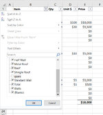
After trying a number of things, my closest solution was to have one sheet as the source data, then a separate worksheet that referenced the source data (So Output!A1 is set to equal Source!A1, etc.) 1, and applied a filter/sort on the output worksheet to remove the blank spaces.
The primary issue I came up against is that I'm hoping to make the formatting of the output worksheet look nice (otherwise all the blanks rows would be fine). If I format the source data, the formatting doesn't carry over into the referenced cells on the output worksheet. Alternatively, I can't seem to format the output to do something like have the headings in bold because the sort order/length of data in each group changes (maybe I just need to work out some complex conditional formating on the output data). The other issue is that I couldn't seem to find a way to get the output table to automatically update after changing the source data (guessing there is some way to force an automatic re-sort/filter?). I can keep plugging along and trying to resolve these issues, but wondering if I'm missing on a smarter/simpler approach.
As another shot of explaining what I am trying to do in a program I'm more familiar with: In Access, I would create a table with the data, then have a report that is set to Group By on the field I want. There are a number of reasons why I'm really trying to get this to work in Excel and not Access for this particular project...
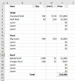
*******Example entry Data (the actual data set and calculations are a lot more complex):*******
******(this data is seperated into rows and columns on the actual worksheet)******
Walls:
Standard Wall 100 @$100 = $10,0000
Half Wall 50 @$30 = $1,500
<empty row if another is needed>
<same empty row if needed another 5 or 10 times....>
Floor:
Big spans 500 @$10 = $5,000
<empty row if another is needed>
<same empty row if needed another 5 or 10 times....>
Roof:
Metal Roof 1,000 @$1 = $1,000
Shinlge Roof 500 @$1 = $ 500
<empty row if another is needed>
<same empty row if needed another 5 or 10 times....>
Totals
Sub Total =$18,000
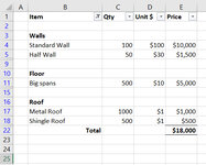
*******Example Output Data (formatted and no unwanted empty rows):*******
Walls:
Standard Wall 100 @$100 = $10,0000
Half Wall 50 @$30 = $1,500
Floor:
Big spans 500 @$10 = $5,000
Roof:
Metal Roof 1,000 @$1 = $1,000
Shinlge Roof 500 @$1 = $ 500
Totals
Sub Total =$18,000
I'm new to the forum, and I did a quick search for similar questions and didn't find anything. I'm sorry if this has been answered before and I missed it.
Thanks!
After trying a number of things, my closest solution was to have one sheet as the source data, then a separate worksheet that referenced the source data (So Output!A1 is set to equal Source!A1, etc.) 1, and applied a filter/sort on the output worksheet to remove the blank spaces.
The primary issue I came up against is that I'm hoping to make the formatting of the output worksheet look nice (otherwise all the blanks rows would be fine). If I format the source data, the formatting doesn't carry over into the referenced cells on the output worksheet. Alternatively, I can't seem to format the output to do something like have the headings in bold because the sort order/length of data in each group changes (maybe I just need to work out some complex conditional formating on the output data). The other issue is that I couldn't seem to find a way to get the output table to automatically update after changing the source data (guessing there is some way to force an automatic re-sort/filter?). I can keep plugging along and trying to resolve these issues, but wondering if I'm missing on a smarter/simpler approach.
As another shot of explaining what I am trying to do in a program I'm more familiar with: In Access, I would create a table with the data, then have a report that is set to Group By on the field I want. There are a number of reasons why I'm really trying to get this to work in Excel and not Access for this particular project...
*******Example entry Data (the actual data set and calculations are a lot more complex):*******
******(this data is seperated into rows and columns on the actual worksheet)******
Walls:
Standard Wall 100 @$100 = $10,0000
Half Wall 50 @$30 = $1,500
<empty row if another is needed>
<same empty row if needed another 5 or 10 times....>
Floor:
Big spans 500 @$10 = $5,000
<empty row if another is needed>
<same empty row if needed another 5 or 10 times....>
Roof:
Metal Roof 1,000 @$1 = $1,000
Shinlge Roof 500 @$1 = $ 500
<empty row if another is needed>
<same empty row if needed another 5 or 10 times....>
Totals
Sub Total =$18,000
*******Example Output Data (formatted and no unwanted empty rows):*******
Walls:
Standard Wall 100 @$100 = $10,0000
Half Wall 50 @$30 = $1,500
Floor:
Big spans 500 @$10 = $5,000
Roof:
Metal Roof 1,000 @$1 = $1,000
Shinlge Roof 500 @$1 = $ 500
Totals
Sub Total =$18,000
I'm new to the forum, and I did a quick search for similar questions and didn't find anything. I'm sorry if this has been answered before and I missed it.
Thanks!
") .
.


