Would like to eliminate #NUM error from my columns

[Gusnk]

Excel Experts –



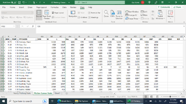
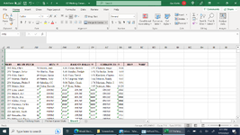
I have two spreadsheets, one with a set of data with 23 columns and over 2,000 rows. Each year there will be additional rows added. I also have ranked each column (category) to provide me top to bottom player performance. I have also correspondingly named each column (category) in a different spreadsheet so I can list the players top to bottom. Some of the categories have criteria that must be met before listing the player. If they do not meet the criteria, they will not be listed. I have used the following formulas to help me achieve this goal, but unfortunately for me it creates errors at the end of the column if the criteria have not been met. I have tried using the following formulas without success.

IF('Pitcher Career Stats'!AR2<>"","",OFFSET('Pitcher Career Stats'!$Z$2,MATCH(SMALL('Pitcher Career Stats'!AR$2:AR$5000,ROW()-ROW(AV$5)+1),'Pitcher Career Stats'!AR$2:AR$5000,0)-1,0))

IF('Pitcher Career Stats'!AS2="",OFFSET('Pitcher Career Stats'!$Z$2,MATCH(SMALL('Pitcher Career Stats'!AS$2:AS$5000,ROW()-ROW(AX$5)+1),'Pitcher Career Stats'!AS$2:AS$5000,0)-1,0),"")

IF('Pitcher Career Stats'!M2>=2000,OFFSET('Pitcher Career Stats'!$Z$2,MATCH(SMALL('Pitcher Career Stats'!AS$2:AS$5000,ROW()-ROW(AX$5)+1),'Pitcher Career Stats'!AS$2:AS$5000,0)-1,0),"")

Once it does not meet the criteria it leaves the following error message in cell #NUM!

Sample of spreadsheet:

HITS / 9

Moyer, Jamie	8.62​
Pettitte, Andy	8.76​
Sabathia, CC	9.04​
Colon, Bartolo	9.17​
#NUM!​	####​

Once the criteria are met is there some way to eliminate the error from appearing?

Thanks in advance for your consideration.

Gus

 

[Sufiyan97]

Try

=IFERROR(IF('Pitcher Career Stats'!M2>=2000,OFFSET('Pitcher Career Stats'!$Z$2,MATCH(SMALL('Pitcher Career Stats'!AS$2:AS$5000,ROW()-ROW(AX$5)+1),'Pitcher Career Stats'!AS$2:AS$5000,0)-1,0),""),"")

 

[Gusnk]

Sufiyan97 -

I appreciate your help, but unfortunately this does not work. I have uploaded 2 images for you to look at. First one is the columns that I use to rank each pitchers stats. The second one is where I would like the output to show.

Image 1:
The formular in column AR is =IF(M2>=2000,(RANK(U2,$U$2:$U$1745,1)+COUNTIF($U$2:U2,U2)-1),"")
This allows me to rank the each player.

Image 2:
Column AV is one of the columns where I am having the issues.

Again, I appreciate your help,

Regards, Gus

 

[Fluff]

How about

=TAKE(SORT(FILTER('Pitcher Career Stats'!Z2:AR5000,'Pitcher Career Stats'!AR$2:AR$5000<>""),19,1),,1)

 

[Gusnk]

Fluff -

Thanks it works perfectly. I just have to remember not to have any data below or to the right. I appreciate all the help I received from the forum.

Best regards,

Gus

 

[Fluff]

You can have data to the right as it should only spill down.

 

[Gusnk]

Fluff -

When I used the formula your provided and I left original data in the right column, the #Spill error appeared completely in the 100 rows. Once I removed the data to the right it filled in correctly. I than replaced the data to the right column.

Best regards,

Gus