Wrangling Joined Salesforce Reports with Pivot Tables

[ExcelCT]

Hello all.

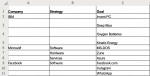
If anyone has used joined reports in Salesforce, you'll know the export output is limited to grouped, pre-formatted Excel sheets that are not (in Salesforce parlance) 'detailed reports'. For using pivot tables with these exports, this is a bit of a problem because there are not repeating rows and rather the data looks like below. The actual report is way more complicated, but I've made a sample of how the data looks. If with your help I can figure out how to get a working pivot table with this sample data, I'm confident I could handle the rest of the work.

About the data: This is the format it comes out of Salesforce. I can image some ways I could get my required output (see below) without using pivot tables - but I love pivot tables and would like to use them if possible. I know I could do some amount of "post processing" via macros or helper columns - and I may have to do that. I would like to keep post-processing to a minimum.



It's important to note that the strategy entries (or lack thereof) and the goals (or lack thereof) are independent of each other. That is the 'join' in Salesforce (in my example, the join is on Company). Thus each company can have 0 to n number of Strategies and 0 to n number of Goals. They have both. They may have neither. Obviously pivot table out of the box can't really deal with this format very well. As humans, it is easy to understand what I'm trying to get to, but not sure how to make a pivot table do this. I do have PowerPivot and have used it somewhat in the past but not an expert user of it. But if there is a PowerPivot-based solution, I could enact that.

Thanks in advance for your help.

-CT

 

[sandy666]

with Excel Table is easier, with named range is a bit complicated because you'll need to transform table in PQ Editor but it will work also

You are welcome
Thanks for the feedback

 

[ExcelCT]

I've got it mostly working on my real data set. The additional columns on my real data has caused one artifact: zero's are no longer showing up like in the sample. Where the count of Strategy and Goals is > 1 the numbers being reported in the pivot are correct. Where there are 100% blanks for a given "company", it is showing 1. So maybe I need to do additional "filldowns" for some of the other columns as well. I'll play with it. But seems close.

CT

 

[sandy666]

sure, let me know if it will work (or not) for you

 

[ExcelCT]

sure, let me know if it will work (or not) for you

It's very strange. Just to test, I chopped out the extra columns to get down to three like the sample. Unfortunately, it didn't make a difference: where I expect to see 0's, I still see a minimum of 1 in the pivot.

Conversely, if I add additional columns to your sample sheet...your sample still correctly shows zeros. Your sample is rock solid no matter what I throw it.

But on my real sheet, even though it looks the same (I've went ahead and chopped it down to only three records and three columns) from how the data is laid out...the pivot table produced still shows '1's where there should be 0s.

So...either I have messed up how to initiate the editor where the code is or even though I created the table with the CTRL+T something is still amiss. Or...? Something else "embedded" in the Salesforce output file that is causing problems I can't visually see?

Not sure.

Here's what I am doing

1) Opening the Salesforce-generated file.
2) Selecting $A$1:$I$5000 (for real, or just a small cut down sample) and doing CTRL-T to define the table.
3) Going to Data tab, select New Query -> From other Data Sources->Blank Query
4) Pasting in your code
5) Changing the references to the 'Company' column to the real name of the column
6) Saving the changes

No errors. The pivot table gets correctly created and all the rows are there. But there are never any zeros for the relevant columns. Always a minimum of 1. Otherwise, the counts look correct in random sampling.

Again, if I take a chunk of my real data and paste it back into the sample, it works fine. Any ideas?

Thanks in advance

CT

 

[sandy666]

You forgot this is not a Pivot Table but Power Query - this is not the same
re-open example and you will see new table with additional Column [Country] then see the M-code for that and compare with previous code
you added column but didn't change code - it doesn't work that way
that is why example should be representative

this is NOT copy/paste solution

 

[ExcelCT]

>>You forgot this is not a Pivot Table but Power Query - this is not the same

I realize they are different. Pardon for the sloppy language.

When you say reopen the example, does that mean you updated post 5?

I am aware the sample should be representative but I guess I didn't think the other columns (would be meaningful, especially since the Power Query allows removal of columns that might not be as needed). Will definitely take a look at the new M-code - I really appreciate it.

But I guess what I was trying to explain before (but may have not done a good job doing!) was that even if I prepare my real file and cut it down to just three columns so that it IS representative...and even if I call the columns exactly the same as the sample...the Power Query produced results table still gives me 1s where I was expecting 0s. But if I take that cut-down representative data and put that into your sample spreadsheet - it gives 0s (correctly). So even with the same data and same columns (that can then use the same m-code) your sample spreadsheet works and mine doesn't. And I'm trying to understand why. I am definitely painting by numbers on Power Query because it's brand new to me. After I reverse engineer how it works and watch some videos and read some tutorials I'll likely get the hang of it.

Thanks for your awesome help from this Power Query n00b

CT

 

[sandy666]

since the Power Query allows removal of columns

like you said: in Power Query not in source data
only in a few cases can this be done in the source table
as you said Power Query n00b who only met PQ in this thread, you are making good progress
when you understand how Power Query works without copy/paste clicks it will be a great day ?

I will wait to see: all works with original data