x-axis calendar week and year for multiple years

[atestacc]

Hello,

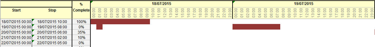
I'd like to change the x-axis with values from the table to generate a Gantt chart.
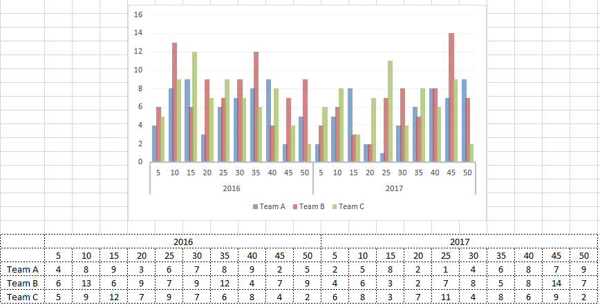
I have no problems to create a chart with for example a range from calendar week 20-51.

<code style="margin: 0px; padding: 0px; font-style: inherit; font-weight: inherit; line-height: 12px;">chtChart.Axes(xlValue).MinimumScale = Sheets("Sheet1").Range("J9")
chtChart.Axes(xlValue).MaximumScale = Sheets("Sheet1").Range("K9")
chtChart.Axes(xlValue).MajorUnit = Sheets("Sheet1").Range("L9")
</code>

I have added some rows to help me to scale the axis (J7 and J9 / K7 and K9).
In those cells, I search for the lowest and highest date and change it to a calendar week.

I also changed the numberFormat to "0 KW" KW means calendar week in German.

[COLOR=#333333][FONT=monospace]chtChart.Axes(xlColumns).TickLabels.NumberFormat = "0 KW"[/FONT][/COLOR][COLOR=#333333]
[/COLOR]

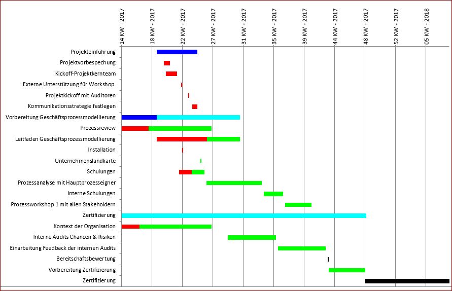
It is working in a range of one year, but as soon as I switch to another year it plots the graph wrong (the reason is obvious week: 42 - 15 makes no sense with this logic right now).

Is there a way to combine week and year and use this to plot the axis (with VBA, because it should be done automatic every time)?

Sadly I can't add files here, one is working because the range is in between (picture 1 and 2) 1-52 and the other isn't working because it switches from 2016-2017-2018 (picture 3 and 4).

http://imageshack.com/a/img923/2558/K5iOcC.png
http://imageshack.com/a/img924/1200/FOQyuy.png

http://imageshack.com/a/img924/1591/FIwvtS.png
http://imageshack.com/a/img922/3849/5DFpbn.png

Additional information:
- Rows A:I are automatically generated (don't touch those please)
- I can add as many "helping" rows as I want.
- Files are in German, VBA in English, if you don't understand something then ask me.


Kind regards,

Niko

 

[Worf]

Welcome to the Forum


You may upload the test workbook to a sharing site like Dropbox and paste a link here.
The pictures below show how to display two-level information for real charts and worksheet Gantt charts.

 

[atestacc]

Welcome to the Forum


You may upload the test workbook to a sharing site like Dropbox and paste a link here.
The pictures below show how to display two-level information for real charts and worksheet Gantt charts.

Hello I've uploaded both test worksheets to Dropbox: https://www.dropbox.com/sh/psy0b2i726urov8/AAC4_VwLGvPtsXiygzDAXaBYa?dl=0

It would be nice if you could check those files. I really don't know how to do this, but your pictures are exactly what I want.

Best regards

 

[Worf]

Hi

I got your workbook and will work on it as soon as possible...

 

[Worf]

Hi Niko

o The new data table (this post)
o The new code (this post)
o The link to my test workbook (next post)
o The final product (next post)


Projektplan

*	J	K	L	M	N	O	P	Q	R
6	Start	End	Range	Arbeitspaket	Start	Duration in KW	Duration in calendar Days	Fertig.grad	still open
7	03/04/17	20/02/18	*	Projekteinführung	08/05/2017	5,714285714	40	40	0
8	42828	43151	*	Projektvorbespechung	15/05/2017	0,857142857	6	6	0
9	14	8	30	Kickoff-Projektkernteam	17/05/2017	1,571428571	11	11	0

<tbody>
</tbody>

Spreadsheet Formulas

Cell Formula J7 =IF(B7="","",MIN(H:H)) K7 =IF(B7="","",MAX(I:I)) M7 =IF(B7="","",B7) N7 =H7 O7 =IF(B7="","",P7/7) P7 =IF(B7="","",(I7-H7)+1) Q7 =IF(B7="","",P7*G7/100) R7 =IF(B7="","",P7-Q7) J8 =IF(B7="","",J7) K8 =IF(B7="","",K7) M8 =IF(B8="","",B8) N8 =H8 O8 =IF(B8="","",P8/7) P8 =IF(B8="","",(I8-H8)+1) Q8 =IF(B8="","",P8*G8/100) R8 =IF(B8="","",P8-Q8) J9 =IF(B7="","",WEEKNUM(J7)) K9 =IF(B7="","",WEEKNUM(K7)) L9 =IF(B7="","",30) M9 =IF(B9="","",B9) N9 =H9 O9 =IF(B9="","",P9/7) P9 =IF(B9="","",(I9-H9)+1) Q9 =IF(B9="","",P9*G9/100) R9 =IF(B9="","",P9-Q9) <tbody> </tbody>

<tbody>
</tbody>

Excel tables to the web >> Excel Jeanie HTML 4

Sub diagramm()
Dim letzteZeile&, ch As Chart, ws As Worksheet, dl!, v As Date, i%
Set ws = Sheets("projektplan")
letzteZeile = ws.Range("H" & Rows.Count).End(xlUp).Row  ' start
Set ch = Charts.Add
With ch
    .Name = "Gantt Chart"
    .ChartType = xlBarStacked
    .PlotVisibleOnly = False
    .SetSourceData Source:=ws.Range("M7:N" & letzteZeile), PlotBy:=xlColumns
    .SeriesCollection(1).Name = "=""invisible"""
    .SeriesCollection.NewSeries
    .SeriesCollection(2).Name = "=""finished"""
    .SeriesCollection(2).Values = "='Projektplan'!$Q$7:$Q" & letzteZeile
    .SeriesCollection.NewSeries
    .SeriesCollection(3).Name = "=""open"""
    .SeriesCollection(3).Values = "='Projektplan'!$R$7:$R" & letzteZeile
End With
ch.SeriesCollection(1).Format.Fill.Visible = False
ch.Legend.Delete
ch.Axes(xlCategory).ReversePlotOrder = True
With ch.Axes(xlValue)
    .MinimumScale = ws.[j7]
    .MaximumScale = ws.[k7]
    .MajorUnit = ws.[l9]
    .TickLabels.Orientation = 89
    .TickLabels.Font.Color = RGB(250, 250, 250)     ' invisible labels
End With
ch.PlotArea.Top = ch.PlotArea.Top + 20
dl = 0
Do While dl < ch.PlotArea.InsideWidth
    With ch.Shapes.AddTextbox(2, ch.PlotArea.InsideLeft - 10 + dl, ch.PlotArea.InsideTop - 70, 20, 70)
        v = CDate(ws.[j7] + dl / ch.PlotArea.InsideWidth * (ws.[k7] - ws.[j7]))
        .TextFrame.Characters.Text = Format(CStr(WorksheetFunction.WeekNum(v)), "00") & " KW - " & CStr(Year(v))
        .TextFrame2.VerticalAnchor = msoAnchorMiddle
        .TextFrame2.HorizontalAnchor = msoAnchorNone
    End With
    dl = dl + ch.PlotArea.InsideWidth * ws.[l9] / (ws.[k7] - ws.[j7])
Loop
With ws
    For i = 7 To .Cells(.Rows.Count, 1).End(xlUp).Row
        If myRegEx(.Cells(i, 1), "[a-zA-Z]{3,5}-\d{2}") Then
                ch.SeriesCollection(2).Points(i - 6).Format.Fill.ForeColor.RGB = RGB(0, 0, 255)
                ch.SeriesCollection(3).Points(i - 6).Format.Fill.ForeColor.RGB = RGB(0, 255, 255)
        ElseIf myRegEx(.Cells(i, 1), "[a-zA-Z]{3,5}-\d{2}-\d{3}") Then
            With ch
                .SeriesCollection(2).Points(i - 6).Format.Fill.ForeColor.RGB = RGB(255, 0, 0)
                .SeriesCollection(3).Points(i - 6).Format.Fill.ForeColor.RGB = RGB(0, 255, 0)
            End With
        ElseIf myRegEx(.Cells(i, 1), "[a-zA-Z]{3,5}-\d{2}-\d{3}-MS\d{1,2}") Then
            With ch
                .SeriesCollection(2).Points(i - 6).Format.Fill.ForeColor.RGB = RGB(0, 0, 0)
                .SeriesCollection(3).Points(i - 6).Format.Fill.ForeColor.RGB = RGB(0, 0, 0)
            End With
        End If
    Next
End With
End Sub

 

[Worf]

https://www.dropbox.com/s/iimke27ysmdc56r/workingENS.xlsm?dl=0

 

[atestacc]

https://www.dropbox.com/s/iimke27ysmdc56r/workingENS.xlsm?dl=0

Thank you sooooo much!!!
It works perfect.
Exactly what I wanted.
Thank you very much for the time you invested into this.

 

[Worf]

You are welcome and thanks for the feedback.