XIRR function with 1 value from another cell

kapvg

New Member
Joined
Jun 30, 2018
Messages
25
Office Version
  1. 365
  2. 2019
  3. 2016
Platform
  1. Windows
Hi,

I am using Excel 2016 and need help using the XIRR formula for the sample data below:
image_2021-01-16_204953.png


In the above sample data, I want to calculate XIRR in column D. It would be great if I could build the formula like =XIRR ((B$2:B3), C3), (A$2:A3), A3)) but unfortunately excel does not work as per my whims :p

I am unable to figure out a proper way to join/concatenate two ranges to use in the formula and the best I was able to build up after searching around for a couple of hours is:
=XIRR(CHOOSE({1,2},OFFSET($B$2,0,0,MATCH($A3,A:A,FALSE)-1,1),VLOOKUP($A3,$A:$C,3,FALSE)),CHOOSE({1,2},OFFSET($A$2,0,0,MATCH($A3,A:A,FALSE)-1,1),VLOOKUP($A3,$A:$A,1,FALSE)))
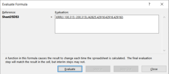
but this does not give the correct result as it ends up taking the value $315 multiple times and same with the date 30-Jun-2017 (takes it 3 times instead of twice) :cry:
image_2021-01-16_211135.png


Without using VBA, is it possible to have a formula created that would work for all cells D3 to D12 (drag down) ??
 

Attachments

  • image_2021-01-16_211042.png
    image_2021-01-16_211042.png
    12.9 KB · Views: 7

Excel Facts

Show numbers in thousands?
Use a custom number format of #,##0,K. Each comma after the final 0 will divide the displayed number by another thousand
I think you want something like the following:

Book1
ABCD
1dateinvestend valueIRR
231-Mar-2017-$100.00$105.00
330-Jun-2017-$200.00$315.0075.17%
430-Sep-2017-$300.00$620.0021.14%
531-Dec-2017-$400.00$861.67-47.34%
631-Mar-2018-$50.00$1,119.1714.23%
730-Jun-2018-$60.00$1,376.6736.05%
830-Sep-2018-$350.00$1,634.1716.69%
931-Dec-2018-$160.00$1,891.6718.93%
1031-Mar-2019-$390.00$2,149.177.59%
1130-Apr-2019-$250.00$2,406.677.32%
1231-May-2019-$90.00$2,664.1714.06%
Sheet1

Array-enter (press ctrl+shift+Enter instead of just Enter) the following formula into D3:

=XIRR(IF(ROW($A$2:A3)=ROW(A3), $C$2:C3)+$B$2:B3, $A$2:A3)

Then copy D3 and paste into D4:D12. Format D3:D12 as Percentage.

Excel surrounds the formulas with curly braces in the Formula Bar to indicate that they were array-entered. Do not type the curly braces yourself.

The following demonstrate the correctness as I interpret the cash flows:

Book1
FGH
1cash flow
231-Mar-2017-$100.00
330-Jun-2017-$200.00
430-Sep-2017-$300.00
531-Dec-2017-$400.00
631-Mar-2018-$50.00
730-Jun-2018-$60.00
830-Sep-2018-$350.00
931-Dec-2018-$160.00
1031-Mar-2019-$390.00
1130-Apr-2019-$250.00
1231-May-2019-$90.00
1331-May-2019$2,664.17
1414.06%IRR
15TRUEG=D?
Sheet1

The formula in G14 is (normally-entered; just press Enter as usual):

=XIRR(G2:G13, F2:F13)
 
Upvote 0
Solution
PS.... I had mean to include the following as another demonstrate of the correctness as I interpret the cash flows. Refer to the first XL2BB snippet in response #2.

xirr multicol vals.xlsx
IJK
1end value
231-Mar-2017$100.00
330-Jun-2017$303.33
430-Sep-2017$613.56
531-Dec-2017$1,034.25
631-Mar-2018$1,118.36
730-Jun-2018$1,215.66
830-Sep-2018$1,606.65
931-Dec-2018$1,820.83
1031-Mar-2019$2,270.87
1130-Apr-2019$2,545.56
1231-May-2019$2,664.17
135.84E-06J-C
Sheet1
Rich (BB code):
Formulas:
J2: =-B2
J3: =J2*(1+$D$12)^((I3-I2)/365) - B3
Copy J3 into J4:J12

Note that for the purpose of applying the XIRR rate, interest is compounded daily.
 
Upvote 0
Array-enter (press ctrl+shift+Enter instead of just Enter) the following formula into D3:

=XIRR(IF(ROW($A$2:A3)=ROW(A3), $C$2:C3)+$B$2:B3, $A$2:A3)
Many thanks joeu2004 !!!
Your formula works perfectly even with the larger data set that I have. ??

I am able to use the above formula for my data set but, unfortunately as I am a noob at this, I am unable to understand how it works (even after going through the 'Evaluate Formula' multiple times).

Can you please kindly explain how this formula works??
 
Upvote 0
Array-enter (press ctrl+shift+Enter instead of just Enter) the following formula into D3:

=XIRR(IF(ROW($A$2:A3)=ROW(A3), $C$2:C3)+$B$2:B3, $A$2:A3)
To revalidate the above, I have confirmed the results with the ArrayUnion UDF and they work perfectly. But as I am unable to use VBA in this excel file, I will go with the formula from joeu2004 and hope someone can help me understand how the formula works?
 
Upvote 0
Can you please kindly explain how this formula works??

For any sequence of cash flows starting on the date in $A$2 and ending on a subsequent date (in A3, A4 etc), the cash flows (inflows) are the corresponding values in column B. But for the end date, we treat the ending value in column C as an additional cash flow (outflow, oppositely signed). So for the sequence of cash flows for the dates in $A$2:A12, for example, the last net cash flow is C12+B12.

The syntax $A$2:A3 keeps $A$2 as the date of the first cash flow, while changing the date of the last cash flow to A3, A4 etc as we copy the formula down the column. Similarly for the ranges $B$2:B3 and $C$2:C3.

The IF expression creates an array of the form {FALSE, FALSE,..., C12} (stylistically; not valid Excel syntax) for the sequence of cash flows for the dates in $A$2:A12.

The condition of the IF expression is an array of the form (again, stylistically) {ROW($A$2)=ROW(A12), ROW(A3)=ROW(A12),..., ROW(A12)=ROW(A12)}, which is TRUE only for the last row.

Thus, the first parameter of the XIRR expression is an array of the form (stylistically) {FALSE+$B$2, FALSE+B3,..., C12+B12}. And in that context, Excel treats FALSE as 0. Thus, the first parameter is an array of the form {$B$2, B3,..., C12+B12)}.

The second XIRR parameter can simply be the corresponding dates, $A$2:A12. No special treatment is needed.

So, stylistically, the XIRR expression becomes XIRR({$B$2, B3,..., C12+B12}, $A$2:A12).

-----

The Excel IRR model assumes that cash flows occur at the end of the period (on the corresponding date), and that interest, compounded daily, is calculated based on the previous balance at the end of the previous period (on the previous date).

This is demonstrated by the amortization schedule in response #3.

In J3, the previous balance plus interest compounded daily is calculated by the expression J2*(1+$D$12)^((I3-I2)/365).

And the end-of-the-period cash flow is added by the expression -B3. We negate the inflow because you choose to represent inflow as negative values, and in the amortization schedule, I choose to represent the current balance as a positive value.

Thus, the ending balance for the sequence of cash flows for the dates in $A$2:A12 is the value in J12, which matches the ending value in C12 in the IRR model in response #2.

-----

You might note that the current balances for the intermediate dates (J3:J11) do not match the ending values in C3:C11 in the IRR model.

That is because the IRR is an average rate, which might (and does) differ from the actual growth rate for any particular sub-period.

In that case, we only expect the first and last balances to match the IRR model.
 
Upvote 0
For any sequence of cash flows starting on the date in $A$2 and ending on a subsequent date (in A3, A4 etc), the cash flows (inflows) are the corresponding values in column B. But for the end date, we treat the ending value in column C as an additional cash flow (outflow, oppositely signed). So for the sequence of cash flows for the dates in $A$2:A12, for example, the last net cash flow is C12+B12.

The syntax $A$2:A3 keeps $A$2 as the date of the first cash flow, while changing the date of the last cash flow to A3, A4 etc as we copy the formula down the column. Similarly for the ranges $B$2:B3 and $C$2:C3.

The IF expression creates an array of the form {FALSE, FALSE,..., C12} (stylistically; not valid Excel syntax) for the sequence of cash flows for the dates in $A$2:A12.

The condition of the IF expression is an array of the form (again, stylistically) {ROW($A$2)=ROW(A12), ROW(A3)=ROW(A12),..., ROW(A12)=ROW(A12)}, which is TRUE only for the last row.

Thus, the first parameter of the XIRR expression is an array of the form (stylistically) {FALSE+$B$2, FALSE+B3,..., C12+B12}. And in that context, Excel treats FALSE as 0. Thus, the first parameter is an array of the form {$B$2, B3,..., C12+B12)}.

The second XIRR parameter can simply be the corresponding dates, $A$2:A12. No special treatment is needed.

So, stylistically, the XIRR expression becomes XIRR({$B$2, B3,..., C12+B12}, $A$2:A12).

-----

The Excel IRR model assumes that cash flows occur at the end of the period (on the corresponding date), and that interest, compounded daily, is calculated based on the previous balance at the end of the previous period (on the previous date).

This is demonstrated by the amortization schedule in response #3.

In J3, the previous balance plus interest compounded daily is calculated by the expression J2*(1+$D$12)^((I3-I2)/365).

And the end-of-the-period cash flow is added by the expression -B3. We negate the inflow because you choose to represent inflow as negative values, and in the amortization schedule, I choose to represent the current balance as a positive value.

Thus, the ending balance for the sequence of cash flows for the dates in $A$2:A12 is the value in J12, which matches the ending value in C12 in the IRR model in response #2.

-----

You might note that the current balances for the intermediate dates (J3:J11) do not match the ending values in C3:C11 in the IRR model.

That is because the IRR is an average rate, which might (and does) differ from the actual growth rate for any particular sub-period.

In that case, we only expect the first and last balances to match the IRR model.
Many thanks for this detailed explanation.

I was not aware that we can use the IF expression in this manner, was a nice learning and hopefully will be able to use it in future scenarios.

With XIRR, I was thinking about XIRR in its traditional sense and was thus expecting to have (number of rows +1) values for both the XIRR (values, dates) segments. I did not realize that as the final/last date is the same, one can easily add the last amount in the 'Invested' column with the amount in the 'Value' column to get a net amount for the last date.?

I have tried and can confirm that as long as an amount in the 'Value' column is populated for the final date, this formula works perfectly even if there is no amount in the 'Invested' column.?
 
Upvote 0
=XIRR(IF(ROW($A$2:A3)=ROW(A3), $C$2:C3)+$B$2:B3, $A$2:A3)

Although that is not wrong, it is unnecessarily complicated. It is sufficient to array-enter:

=XIRR(IF(ROW($A$2:A3)=ROW(A3), C3)+$B$2:B3, $A$2:A3)

The point is: since ROW($A$2:A3)=ROW(A3) is true only for the last row of the term $A$2:A3, only the last row of the term $C$2:C3 is used, namely C3.
 
Upvote 0

Forum statistics

Threads
1,214,979
Messages
6,122,551
Members
449,088
Latest member
davidcom

We've detected that you are using an adblocker.

We have a great community of people providing Excel help here, but the hosting costs are enormous. You can help keep this site running by allowing ads on MrExcel.com.
Allow Ads at MrExcel

Which adblocker are you using?

Disable AdBlock

Follow these easy steps to disable AdBlock

1)Click on the icon in the browser’s toolbar.
2)Click on the icon in the browser’s toolbar.
2)Click on the "Pause on this site" option.
Go back

Disable AdBlock Plus

Follow these easy steps to disable AdBlock Plus

1)Click on the icon in the browser’s toolbar.
2)Click on the toggle to disable it for "mrexcel.com".
Go back

Disable uBlock Origin

Follow these easy steps to disable uBlock Origin

1)Click on the icon in the browser’s toolbar.
2)Click on the "Power" button.
3)Click on the "Refresh" button.
Go back

Disable uBlock

Follow these easy steps to disable uBlock

1)Click on the icon in the browser’s toolbar.
2)Click on the "Power" button.
3)Click on the "Refresh" button.
Go back
Back
Top