XLOOKUP Help

tim220225

New Member
Joined
Jun 4, 2012
Messages
29
Office Version
  1. 365
Platform
  1. Windows
Hello, I need some help with XLOOKUP. I am tasked with making this worksheet pull data that corresponds with the number of divisions in cell (G3). I have tried multiple ideas and can't get the results I need. I now have it partially working up to 43 divisions as in the image attached. I need to adjust my current formula to return the first three columns to the right of the number of divisions higher than 43. For the life of me I can't get it to work. What is in yellow is how I need it to display.

Thanks for the help!
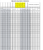

Index Head.png
 

Excel Facts

Why are there 1,048,576 rows in Excel?
The Excel team increased the size of the grid in 2007. There are 2^20 rows and 2^14 columns for a total of 17 billion cells.
Can you upload with Xl2BB? Its a very nice tool and much easier to see your data and current formulas. Also you should update your profile to incorporate what version of excel you are using.
 
Upvote 0
Hi, try this formula
=IFERROR(XLOOKUP(G3,A6:A47,B6:D47),IFERROR(XLOOKUP(G3,E6:E47,F6:H47),IFERROR(XLOOKUP(G3,I6:I47,J6:L47),XLOOKUP(G3,M6:M47,N6:P47))))
 
Upvote 0
Can you upload with Xl2BB? Its a very nice tool and much easier to see your data and current formulas. Also you should update your profile to incorporate what version of excel you are using.
I have tried to install this tool. I’m going to have to work on it more.
 
Upvote 0
Hi, try this formula
=IFERROR(XLOOKUP(G3,A6:A47,B6:D47),IFERROR(XLOOKUP(G3,E6:E47,F6:H47),IFERROR(XLOOKUP(G3,I6:I47,J6:L47),XLOOKUP(G3,M6:M47,N6:P47))))
That solution works! I was using a similar formula without the IFERROR. I need to work with this formula to understand how the addition of IFERROR made it work.

Thank you very much!
 
Upvote 0
As Xlookup has it's own built error handling, you don't need iferror, you can use
Excel Formula:
=XLOOKUP(G3,A6:A47,B6:D47,XLOOKUP(G3,E6:E47,F6:H47,XLOOKUP(G3,I6:I47,J6:L47,XLOOKUP(G3,M6:M47,N6:P47,""))))
 
Upvote 0
Solution
As Xlookup has it's own built error handling, you don't need iferror, you can use
Excel Formula:
=XLOOKUP(G3,A6:A47,B6:D47,XLOOKUP(G3,E6:E47,F6:H47,XLOOKUP(G3,I6:I47,J6:L47,XLOOKUP(G3,M6:M47,N6:P47,""))))
Thank you! This works and is cleaner.
 
Upvote 0
Glad we could help & thanks for the feedback.
 
Upvote 0

Forum statistics

Threads
1,214,787
Messages
6,121,558
Members
449,038
Latest member
Guest1337

We've detected that you are using an adblocker.

We have a great community of people providing Excel help here, but the hosting costs are enormous. You can help keep this site running by allowing ads on MrExcel.com.
Allow Ads at MrExcel

Which adblocker are you using?

Disable AdBlock

Follow these easy steps to disable AdBlock

1)Click on the icon in the browser’s toolbar.
2)Click on the icon in the browser’s toolbar.
2)Click on the "Pause on this site" option.
Go back

Disable AdBlock Plus

Follow these easy steps to disable AdBlock Plus

1)Click on the icon in the browser’s toolbar.
2)Click on the toggle to disable it for "mrexcel.com".
Go back

Disable uBlock Origin

Follow these easy steps to disable uBlock Origin

1)Click on the icon in the browser’s toolbar.
2)Click on the "Power" button.
3)Click on the "Refresh" button.
Go back

Disable uBlock

Follow these easy steps to disable uBlock

1)Click on the icon in the browser’s toolbar.
2)Click on the "Power" button.
3)Click on the "Refresh" button.
Go back
Back
Top