XLOOKUP - how to extend the 'If not found' argument to the return array?

[Chazzo]

Hello All,

Is there a way to have the 'If_not_found' argument extended so that it populates all cells to the return array?

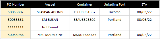
For example, I would like to have the text string "Not Found" spill to range I:K in my example below.

By default, it appears that it will only fill the left most column.

My formula is written in H2 and is as follows: =XLOOKUP(G2,A:A,B:E,"Not Found")

Is it possible to have the formula return the 'if not found' input to all of the cells in the return array vs the left most column only?

Thank you in advance...

 

[Fluff]

I suggest that you update your Account details (or click your user name at the top right of the forum) so helpers always know what Excel version(s) & platform(s) you are using as the best solution often varies by version. (Don’t forget to scroll down & ‘Save’)

How about

=XLOOKUP(G2,A:A,B:E,{"Not Found","Not Found","Not Found"})

 

[Chazzo]

I suggest that you update your Account details (or click your user name at the top right of the forum) so helpers always know what Excel version(s) & platform(s) you are using as the best solution often varies by version. (Don’t forget to scroll down & ‘Save’)

How about

=XLOOKUP(G2,A:A,B:E,{"Not Found","Not Found","Not Found"})

Thanks Fluff,

I updated my account details to show that I'm using 365. Your solution certainly works and I have taken note. I thought there may be a way to have the argument spill over the same way the the matches would within the range. I appreciate the quick feedback!

 

[Fluff]

Glad to help & thanks for the feedback.

 

[Peter_SSs]

I thought there may be a way to have the argument spill over the same way the the matches would within the range.

You could try these, particularly if it needs to spill over a lot of columns.

=XLOOKUP(G2,A:A,B:E,INDEX("not found",SEQUENCE(,COLUMNS(B:E),,0)))

=XLOOKUP(G2,A:A,B:E,MAKEARRAY(1,COLUMNS(B:E),LAMBDA(r,c,"not found")))

 

[Chazzo]

You could try these, particularly if it needs to spill over a lot of columns.

=XLOOKUP(G2,A:A,B:E,INDEX("not found",SEQUENCE(,COLUMNS(B:E),,0)))

=XLOOKUP(G2,A:A,B:E,MAKEARRAY(1,COLUMNS(B:E),LAMBDA(r,c,"not found")))

Thanks Peter!

This is closer to what I was looking for. The first formula works great, couldn’t get the second one to work but I have what I need.

Thanks again!

 

[Peter_SSs]

This is closer to what I was looking for.

But not exactly??

couldn’t get the second one to work

If you got a #NAME? error then it probably means that you have updates to Office that have not been applied. If it was something else that went wrong I would be interested to know what it was as the two formulas produced identical results for me.

Thanks Peter!

You're welcome.