Xlookup Starting Point

[OKCIrish]

Hello,

I'm new to excel, however I am very good at solving issues if I can get going in the right direction or have previous formulas to work off of or modify. I am having trouble on how to solve/approach this data point I would like returned to me.

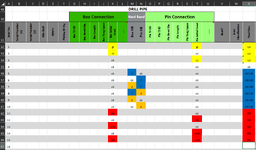
My main data point that needs to be returned to a specific text in column X is OK, OK-HB, RPR or REJ is based on what is inputted in column K, M, N, T & V, from either drop-down menu selected or manually inputted.

I have been told a nested if formula would cause a lot of complications and Xlookup would be a better suit. However, I am stuck on how I should approach this table for Xlookup to work correctly. Do I have to have all different kinds of variations on the table, or can there be key components for the formulas to look up and return?

In column K & T if the drop down or manual input of STS or UND is selected then it overrides everything and the text in column X comes up as REJ.
Then column K, T, and V would compare for special text in column K & T and column V would have an X in it and column X would be returned as RPR if any of those parameters are met.
After that column K, T, M & N would be looked at. Column K & T would have to have either OK or OK-FR then column M & N would have F or D in it and then column X would return with OK-HB
And finally if column K, M, N, T & V have OK or OK-FR then column X would be returned as OK, with the variance of sometimes column N not having OK in the column at all but still returning column X with OK.

I would greatly appreciate any leads on how to approach this.

 

[OKCIrish]

so, is what you have above the criteria you want? Just to confirm, please.

Yes

 

[awoohaw]

Ok, Im not sure if you'll be able to plug and play this, but it should give you a working point:
First I created named ranged for the XLOOKUP and MATCH FUNCTIONS These are on the worksheet "Named Ranges".
Then the MAIN worksheet has data validation at a high level for each column. By high level, I mean the drop downs for M,N are not filtered for items in K or T. Also, i have some Zeros in the lists, those can be deleted.

It isn't conditional formating, but the resulting calcuation with give an error in column X if information is not input correctly.

XLookup for OKCIrish.xlsx
	A	B	C	D	E	F	G	H	I	J	K	L
1	K-Box Initial Condition	M-Box Hard Band	N-Pin HB	T-Pin Initial Cond	V-Bent	Map X to		KBOXINTLIST	MBOXHARDLIST	NPINLIST	TPINLIST	VBENTLIST
2	BM				X	RPR		0	0	0	0	0
3	BM					RPR		BM	D	D	BM	X
4	BV				X	RPR		BV	F	F	BV
5	BV					RPR		CS			CS
6	CS				X	RPR		CT			CT
7	CS					RPR		DIM			DIM
8	CT				X	RPR		GS			GS
9	CT					RPR		GT			GT
10	DIM				X	RPR		MRF			MRF
11	DIM					RPR		OK			OK
12	GS				X	RPR		OK-FR			OK-FR
13	GS					RPR		PIT			PIT
14	GT				X	RPR		PS			PS
15	GT					RPR		PUT			PUT
16	MRF				X	RPR		SC			SC
17	MRF					RPR		SD			SD
18	OK	F				OK		STS			STS
19	OK		F			OK		UND			UND
20	OK-FR	D				OK		UNS			UNS
21	OK-FR		D			OK		WO			WO
22	PIT				X	RPR		WT			WT
23	PIT					RPR
24	PS				X	RPR
25	PS					RPR
26	PUT				X	RPR
27	PUT					RPR
28	SC				X	RPR
29	SC					RPR
30	SD				X	RPR
31	SD					RPR
32	STS					REJ
33	UND					REJ
34	UNS				X	RPR
35	UNS					RPR
36	WO				X	RPR
37	WO					RPR
38	WT				X	RPR
39	WT					RPR
40				BM	X	RPR
41				BV	X	RPR
42				CS	X	RPR
43				CT	X	RPR
44				DIM	X	RPR
45				GS	X	RPR
46				GT	X	RPR
47				MRF	X	RPR
48				PIT	X	RPR
49				PS	X	RPR
50				PUT	X	RPR
51				SC	X	RPR
52				SD	X	RPR
53				UNS	X	RPR
54				WO	X	RPR
55				WT	X	RPR
56				BM		RPR
57				BV		RPR
58				CS		RPR
59				CT		RPR
60				DIM		RPR
61				GS		RPR
62				GT		RPR
63				MRF		RPR
64				OK		OK-HB
65				OK		OK-HB
66				OK-FR		OK-HB
67				OK-FR		OK-HB
68				PIT		RPR
69				PS		RPR
70				PUT		RPR
71				SC		RPR
72				SD		RPR
73				STS		REJ
74				UND		REJ
75				UNS		RPR
76				WO		RPR
77				WT		RPR
Named Ranges

XLookup for OKCIrish.xlsx
											K		M	N						T		V		X		Z
1													Hard Band
2											Box Initial Cond.		Box HB	Pin HB						Pin Initial Cond.		Bent?		Final Class		Comments
3											BM													RPR
4											CS													RPR
5											BM											X		RPR
6											CT													RPR
7											OK		F											OK
8											BM													RPR
9											BM													RPR
10											OK-FR			D										OK
11											BM													RPR
12											UND													REJ
13											BM													RPR
14											BM													RPR
15											BM													RPR
16											BM													RPR
17											BM													RPR
18											BM													RPR
19
MainSheet for OKCIrish

Cell Formulas
Range	Formula
X3:X18	X3	=INDEX( +Map_X_to, MATCH(K3&M3&N3&T3&V3,K_Box_Initial_Condition&M_Box_Hard_Band&N_Pin_HB&T_Pin_Initial_Cond&V_Bent,0),1)

Named Ranges
Name	Refers To	Cells
K_Box_Initial_Condition	='Named Ranges'!$A$2:$A$77	X3:X18
M_Box_Hard_Band	='Named Ranges'!$B$2:$B$77	X3:X18
Map_X_to	='Named Ranges'!$F$2:$F$77	X3:X18
N_Pin_HB	='Named Ranges'!$C$2:$C$77	X3:X18
T_Pin_Initial_Cond	='Named Ranges'!$D$2:$D$77	X3:X18
V_Bent	='Named Ranges'!$E$2:$E$77	X3:X18

Cells with Data Validation
Cell	Allow	Criteria
K3:K18	List	=KBOXINTLIST
T3:T18	List	=TPINLIST
V3:V18	List	=VBENTLIST
M3:M18	List	=MBOXHARDLIST
N3:N18	List	=NPINLIST

 

[OKCIrish]

Ok, Im not sure if you'll be able to plug and play this, but it should give you a working point:
First I created named ranged for the XLOOKUP and MATCH FUNCTIONS These are on the worksheet "Named Ranges".
Then the MAIN worksheet has data validation at a high level for each column. By high level, I mean the drop downs for M,N are not filtered for items in K or T. Also, i have some Zeros in the lists, those can be deleted.

It isn't conditional formating, but the resulting calcuation with give an error in column X if information is not input correctly.

XLookup for OKCIrish.xlsx
	A	B	C	D	E	F	G	H	I	J	K	L
1	K-Box Initial Condition	M-Box Hard Band	N-Pin HB	T-Pin Initial Cond	V-Bent	Map X to		KBOXINTLIST	MBOXHARDLIST	NPINLIST	TPINLIST	VBENTLIST
2	BM				X	RPR		0	0	0	0	0
3	BM					RPR		BM	D	D	BM	X
4	BV				X	RPR		BV	F	F	BV
5	BV					RPR		CS			CS
6	CS				X	RPR		CT			CT
7	CS					RPR		DIM			DIM
8	CT				X	RPR		GS			GS
9	CT					RPR		GT			GT
10	DIM				X	RPR		MRF			MRF
11	DIM					RPR		OK			OK
12	GS				X	RPR		OK-FR			OK-FR
13	GS					RPR		PIT			PIT
14	GT				X	RPR		PS			PS
15	GT					RPR		PUT			PUT
16	MRF				X	RPR		SC			SC
17	MRF					RPR		SD			SD
18	OK	F				OK		STS			STS
19	OK		F			OK		UND			UND
20	OK-FR	D				OK		UNS			UNS
21	OK-FR		D			OK		WO			WO
22	PIT				X	RPR		WT			WT
23	PIT					RPR
24	PS				X	RPR
25	PS					RPR
26	PUT				X	RPR
27	PUT					RPR
28	SC				X	RPR
29	SC					RPR
30	SD				X	RPR
31	SD					RPR
32	STS					REJ
33	UND					REJ
34	UNS				X	RPR
35	UNS					RPR
36	WO				X	RPR
37	WO					RPR
38	WT				X	RPR
39	WT					RPR
40				BM	X	RPR
41				BV	X	RPR
42				CS	X	RPR
43				CT	X	RPR
44				DIM	X	RPR
45				GS	X	RPR
46				GT	X	RPR
47				MRF	X	RPR
48				PIT	X	RPR
49				PS	X	RPR
50				PUT	X	RPR
51				SC	X	RPR
52				SD	X	RPR
53				UNS	X	RPR
54				WO	X	RPR
55				WT	X	RPR
56				BM		RPR
57				BV		RPR
58				CS		RPR
59				CT		RPR
60				DIM		RPR
61				GS		RPR
62				GT		RPR
63				MRF		RPR
64				OK		OK-HB
65				OK		OK-HB
66				OK-FR		OK-HB
67				OK-FR		OK-HB
68				PIT		RPR
69				PS		RPR
70				PUT		RPR
71				SC		RPR
72				SD		RPR
73				STS		REJ
74				UND		REJ
75				UNS		RPR
76				WO		RPR
77				WT		RPR
Named Ranges

XLookup for OKCIrish.xlsx
											K		M	N						T		V		X		Z
1													Hard Band
2											Box Initial Cond.		Box HB	Pin HB						Pin Initial Cond.		Bent?		Final Class		Comments
3											BM													RPR
4											CS													RPR
5											BM											X		RPR
6											CT													RPR
7											OK		F											OK
8											BM													RPR
9											BM													RPR
10											OK-FR			D										OK
11											BM													RPR
12											UND													REJ
13											BM													RPR
14											BM													RPR
15											BM													RPR
16											BM													RPR
17											BM													RPR
18											BM													RPR
19
MainSheet for OKCIrish

Cell Formulas
Range	Formula
X3:X18	X3	=INDEX( +Map_X_to, MATCH(K3&M3&N3&T3&V3,K_Box_Initial_Condition&M_Box_Hard_Band&N_Pin_HB&T_Pin_Initial_Cond&V_Bent,0),1)

Named Ranges
Name	Refers To	Cells
K_Box_Initial_Condition	='Named Ranges'!$A$2:$A$77	X3:X18
M_Box_Hard_Band	='Named Ranges'!$B$2:$B$77	X3:X18
Map_X_to	='Named Ranges'!$F$2:$F$77	X3:X18
N_Pin_HB	='Named Ranges'!$C$2:$C$77	X3:X18
T_Pin_Initial_Cond	='Named Ranges'!$D$2:$D$77	X3:X18
V_Bent	='Named Ranges'!$E$2:$E$77	X3:X18

Cells with Data Validation
Cell	Allow	Criteria
K3:K18	List	=KBOXINTLIST
T3:T18	List	=TPINLIST
V3:V18	List	=VBENTLIST
M3:M18	List	=MBOXHARDLIST
N3:N18	List	=NPINLIST

Thank you so much for this. I'll should be able to figure it out from here. I just needed a starting point to work off of.

 

[awoohaw]

My pleasure.