XLOOKUP, VLOOKUP, HLOOKUP and INDEX, MATCH

ozzborn

Board Regular
Joined
Sep 14, 2011
Messages
84
Office Version
  1. 365
  2. 2019
  3. 2016
Platform
  1. Windows
I use Excel 365 and Windows 11.

I am trying to create a meeting dashboard to track important meetings for my supervisor. I have a main data set sheet1 that looks like the first picture

I want to develop a formula that I can organize them into a spreadsheet that shows meetings occurring Today, This Week, and Next Week.

I have tried various formulas but it is when I try and integrate the date function that gets me confused.
One other condition is there can be up to 4 Topics scheduled on the same date. My formula would stop working after it found the 1st date.

Sheet1.PNG


The meetings are scheduled randomly and will not be in order ..... however the meetings are always Tue, Wed, and Fri.
It represent a review process that depending the the topic where it enters into the process.

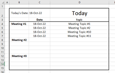
This example below show one example of the Today table where it show all meeting schedule for "Today"
Meeting #2 and Meeting #3 will be blank in this example but if the Today's date was Oct 19th then it would show
all scheduled Topics for Meeting #2.


This example shows the This Week Table where is shows all meetings scheduled for the current work week.

Sheet2_ThisWeek.PNG


Finally the next table shows the "next week" shows all meetings scheduled the next week.
These of course will change based on the Today's date ....and as the meetings are scheduled.
The meetings are often changed and deleted depending on the what is validated and at what meeting.

Sheet2_NextWeek.PNG


Thanks in advance for any help someone might be able to lend.
Ozz
 

Attachments

  • Sheet2_Today.PNG
    Sheet2_Today.PNG
    16 KB · Views: 5

Excel Facts

Select a hidden cell
Somehide hide payroll data in column G? Press F5. Type G1. Enter. Look in formula bar while you arrow down through G.
Maybe something like this?

Book1
ABCD
1Meeting 1Meeting 2Meeting 3
2TueWedFri
310/18/202211/16/202212/9/2022Topic 1
410/18/20229/21/2022Topic 2
510/25/202218-OctTopic 3
610/25/2022Topic 4
711/8/202212/7/20221/6/2023Topic 5
811/30/202212/16/2022Topic 6
910/11/2022Topic 7
1010/19/202210/21/2022Topic 8
1110/26/202210/28/2022Topic 9
1210/18/202210/28/2022Topic 10
1310/18/202210/26/202210/28/2022Topic 11
1411/15/2022Topic 12
15
16
17
18Todays Date10/18/2022
19Meeting 1Topic
2010/18/2022Topic 1
2110/18/2022Topic 2
2210/18/2022Topic 10
2310/18/2022Topic 11
24  
25Meeting 2 
2610/18/2022Topic 3
27  
28  
29  
30Meeting 3 
31  
32
Sheet1
Cell Formulas
RangeFormula
A20:A23A20=IFERROR(FILTER($A$3:$A$14,$A$3:$A$14=$B$18),"")
B20:B23B20=IFERROR(FILTER($D$3:$D$14,$A$3:$A$14=$B$18),"")
A24,B24:B25,B27:B30,A27:A29A24=IFERROR(INDEX(A$3:A$14,AGGREGATE(15,6,(ROW($A$3:$A$14)-ROW($A$3)+1)/(ISNUMBER(MATCH($A$3:$A$14,$B$18,0))),ROWS(B$18:B22))),"")
A26A26=IFERROR(FILTER($B$3:$B$14,$B$3:$B$14=$B$18),"")
B26B26=IFERROR(FILTER($D$3:$D$14,$B$3:$B$14=$B$18),"")
A31A31=IFERROR(FILTER($C$3:$C$14,$C$3:$C$14=$B$18),"")
B31B31=IFERROR(FILTER($D$3:$D$14,$C$3:$C$14=$B$18),"")
Dynamic array formulas.
 
Upvote 0
Solution
Let me look at this. That was fast.

The problem I am having is the primary Data set in on Sheet1 and the other tables are on Sheet2.

Trying to apply the difference.
 
Upvote 0
Ignore A24 must have been a carried over formula.
 
Upvote 0
Ok, I was wondering about A24.

A20 I am getting a #SPILL! message
A21 I am getting a #SPILL! message
A22 I am getting a #SPILL! message
A23 I am getting 18 OCT not sure why.

Next is range B20-B23
 
Upvote 0
Ok this is formula based on my Spreadsheet cells.

A20 =IFERROR(FILTER(Sheet1!$B$3:$B$14,Sheet1!$B$3:$B$14=$C$2),"") and it does not seem to be working result is " #SPILL! "
B20 =IFERROR(FILTER(Sheet1!$E$3:$E$14,Sheet1!$B$3:$B$14=$C$2),"") and it does not seem to be working result is restated formula " =IFERROR(FILTER(Sheet1!$E$3:$E$14,Sheet1!$B$3:$B$14=$C$2),"")


Somehow one of my examples did not get included with the original post. Not sure it makes much deafferents.


Sheet2_Today.PNG
 
Upvote 0
Can you post with a snip with XLB22 by chance? This way its easier to diagnose the issue. SPILL usually happens because you don't have enough space for the data to auto populate with the function. Do you have any data or other formulas?
 
Upvote 0
Clear all cells from A20 & below & then re-enter the formula in A20 only (do NOT use Ctl Shift Enter)
For B20 change the cell to General & then re-enter the formula.
 
Upvote 0
Fluff / Keef2

Fluff, that worked cleaned up the formulas and bingo it populated.

Keef2. thank you for responding so quick and the initial formulas, pretty slick.

Ozz
 
Upvote 0
Keef2, can you recommend the best method to learn quickly how to post with XLB22?
 
Upvote 0

Forum statistics

Threads
1,214,590
Messages
6,120,423
Members
448,961
Latest member
nzskater

We've detected that you are using an adblocker.

We have a great community of people providing Excel help here, but the hosting costs are enormous. You can help keep this site running by allowing ads on MrExcel.com.
Allow Ads at MrExcel

Which adblocker are you using?

Disable AdBlock

Follow these easy steps to disable AdBlock

1)Click on the icon in the browser’s toolbar.
2)Click on the icon in the browser’s toolbar.
2)Click on the "Pause on this site" option.
Go back

Disable AdBlock Plus

Follow these easy steps to disable AdBlock Plus

1)Click on the icon in the browser’s toolbar.
2)Click on the toggle to disable it for "mrexcel.com".
Go back

Disable uBlock Origin

Follow these easy steps to disable uBlock Origin

1)Click on the icon in the browser’s toolbar.
2)Click on the "Power" button.
3)Click on the "Refresh" button.
Go back

Disable uBlock

Follow these easy steps to disable uBlock

1)Click on the icon in the browser’s toolbar.
2)Click on the "Power" button.
3)Click on the "Refresh" button.
Go back
Back
Top